Karyotype of ten fibroblasts after Alu sequences and telomeres hybridization

The image bellow  was obtain after sequential hybridization of telomeric PNA probe (FITC:green) followed by hybridization of Alu-PCR product (Rhodamin: Red):

Pairs of chromosomes are ordered by columns from HSA 1 (left) to XY (right) . Metaphases are ordered by row.

Image acquisition was performed with a low resolution 8bits camera mounted on a Leica DMRB fluorescence microscope (100x). Raw images were transferred from a Unix Cytovision station with 3 inch 1/2 floppy disk to a power Macintosh 9500.

Example of a metaphase after alignment of Alu image on DAPI / telomeres images:

Alu images were aligned on DAPI by hand using Photoshop 3 (Here no background correction, nor contrast enhancement)

Whole chromosome painting was also performed sequentially,  simultaneously on HSA-13 and HSA-6 and HSA-X:

Karyotyping:

Combining R bands (Alu), G bands (DAPI) and chromosomal painting allows to classify chromosomes in a karyogram:

Left:R Bands (Alu sequences). Right: G bands (Inverse DAPI+DoG filter).

2164 full resolution pairs of synthetic images of two overlapping chromosomes

After having fixed the groundtruth images of the "13434" dataset, an older but full resolution dataset, has to be repaired too.

Repair of the "overlapping_chromosomes_examples.h5" dataset:

This dataset contained originally 2854 (grayscaled+groundtruth) pairs of 190x189 images, stored in a unique numpy array. Its shape was 2854x190x189x2.

The grayscaled images could suffer from two problems:

• Some grayscaled images components had black dots: those images were removed (with their corresponding groundtruth labels).

• The images dtype was int64, it is now np.uint8

The overlapping domain is also now more realistic compared with real overlapping chromosomes:

The labels of the groundtruth don't have no more spurious pixels:

Dataset format:

Once downloaded, the dataset shape is (2164, 190, 189, 2) available as:

• an hdf5 file
• a compressed (.npz) numpy array

Download the dataset with a jupyter notebook:

 

 

100 overlapping, full resolution, chromosomes isolated from 14 metaphases of human lymphocytes

Metaphasics chromosomes were hybrized with a PNA telomeric probe (CCCTAA-Cy3) and an additional oligo DNA probe (Cy5) for testing purposes.

100 overlapping chromosomes can be found in that dataset (jpp21). The dataset consists of 12 bits raw greyscaled images available on the DeepFISH repository. The images of overlapping chromosomes were isolated and converted into 8bits rgb images:

Sample of 100 overlapping chromosomes (full resolution)

The overlapping images are also available as combination of DAPI and Cy3 components:

Combination DAPI+Cy3 images (inversed greyscale)

• link to the color images
• link to the greyscaled images 
• link to the notebook

Generating images of overlapping chromosomes

Generating examples of two overlapping chromosome from single chromosomes: 

Notebook:

A notebook showing the different steps to generate overlapping examples is available on kaggle. As well as the raw images.

The idea:

Images of single chromosomes hybridized with with telomeric Cy3-probe and DAPI counterstained were extracted from the image of a metaphase:

DAPI stained chromesomes (left), (CCCTAA)3-PNA-Cy3  probes (Red)

The monochrome DAPI and Cy3 images were added. Single chromosomes were isolated:

All images are 131x128

Given two single chromosomes, examples of overlapping chromosomes were generated combining rotations and translations:

Each greyscale image of a pair of overlapping chromosomes, is associated with a mask containing labels. The pixels of value equal to 3 maps to the overlapping domain of the two chromosomes:

Then a dataset containing 2853 examples of overlapping chromosomes was generated and saved as a h5f file available here:

 examples of overlapping chromosomes 

Once downloaded and uncompressed, the examples can be loaded as a hdf5 file as shown bellow:

Correction of uneven illumination of images of cattle nuclei at low magnification

Looking for a geodesic distance to resolve touching chromosomes

In the previous post, from a cluster of touching mouse chromosomes:

DAPI stained mouse chromosomes

points belonging to negatively curved domains of a contour can be isolated :

To separate the chromosomes, it is tempting to cut between the closest pairs of points.

Python provides itertools.combinations(); the closest pairs of points are in the set of the combinations of every pairs of points:

Each line shows the euclidian distance between two points, the four shortest lines correspond more or less to the contact domains between the chromosomes, cuting along them provides a way to separate the chromosomes.

It should be possible to do better by using a geodesic distance between the points, that is using a path inside the cluster of chromosomes. In the following example: two paths (depending on the chosen pixel neighborhood) between the two blue points were overlaid on a binary image (background is set to 255 and the foreground to 0).

the cluster contourthe cluster contour

 The path were determined as follow using skimage 0.8dev:

graph.route_through_array(negbin ,p1,p2,fully_connected=False)

 or

 graph.route_through_array(negbin ,p1,p2,fully_connected=True)

 with negbin, the negative binary image and p1, p2 the two points figured in blue.

If the background (0) is set to 255 (white) in the grey scale image:

 the path (red) between the two points can be determined by minimizing the "greyscale cost", that is through the valleys between the two points is the image is viewed as a landscape.

All the paths can be determined (blue):Those paths in blue were obtained from the previous binary image:

The paths were sorted according to their cost :

 The four paths with the smallest cost are figured in red, they are "inside" the cluster. Some paths are partially "outside" the cluster and thus are not geodesic routes inside the cluster.
Now if paths are calculated from a 8 bits greyscale image where the background was set to 255 (a naïve idea supposed to prevent a path to go "outside" a cluster):

some routes between two points, go along the contour. The two first routes to with the smallest costs do correspond to touching domains between the chromosomes. However when routes with higher cost are selected:

some correspond to the cluster contour and not to contact domains between the chromosomes, because the cost (sum of pixels grey value) along the contour is probably lower than the cost of a shorter path which have to climb over a contact domain between two chromosomes.

Additional features may distinguish routes belonging to contour from those providing solution to separate chromosomes:

red route on the right resolve touching chromosomes

Minimal cost routes are still better to separate chromosomes than routes obtained with euclidian distance:

The shortest path (on the right) cuts inside the chromosome

Download code

Trying to separate touching mouse chromosomes

In the previous post, from a cluster of touching mouse chromosomes:

points belonging to negatively curved domains of a contour can be isolated :

Yellow points belong to negatively curved domains of the contour.

To separate the chromosomes, it is tempting to cut between the closest pairs of points.

Let's make combination of pairs of points belonging to the contour:

Python provides itertools.combinations(); the closest pairs of points are in the set of the combinations of every pairs of points:

Path between two points belonging to the countour:

Each line shows the euclidian distance between two points, the four shortest lines correspond more or less to the contact domains between the chromosomes, cuting along them provides a way to separate the chromosomes.

It should be possible to do better by using a geodesic distance between the points, that is using a path inside the cluster of chromosomes. In the following example:

On the left, two paths (depending on the chosen pixel neighborhood) between the two blue points were overlaid on a binary image (background is set to 255 and the foreground to 0). The path were determined as follow using skimage 0.8dev:

graph.route_through_array(negbin ,p1,p2,fully_connected=False)

 or

 graph.route_through_array(negbin ,p1,p2,fully_connected=True)

• negbin: the negative binary image
• p1, p2: the two points figured in blue.

On the right the background (0) was set to 255 (white), the path (red) between the two points was determined by minimizing the "greyscale cost", that is through the valleys between the two points is the image is viewed as a greyscaled landscape.

All the paths can be determined (left), and then the paths can be sorted according to their cost (right). The four paths with the smallest cost are figured in red (left).

Download code.

or see bellow:

Telomeres quantification in a nucleus

Telomeres quantification can be done at low magnification in interphasic cells. A microscopic field was recorded with a CCD camera at low magnification (objective x25). Nuclei were counterstained with DAPI and the telomeres were detected with a Cy3-PNA probe.

From the field image, a nucleus is segmented and the DAPI and Cy3 spectral components are isolated. Even at low magnification, the telomeric spots can be segmented as follow:

Background is removed by top-hat filtering with a small structuring element (a disk of size=5). The top-hat image is then submitted to a hmin operator, leaving the peaks higher than 200 gray level units, then regional maxima are found.

The regional maxima are labelled to obtain markers for the watershed algorithm. Once thresholded, the top hat image is converted into distance map using euclidian or chess-board distance without significant difference.

Watershed doesn't succeed very well in separating spots belonging to the lower cluster of three spots. It may be interesting to use a high pass filtered image to build a  distance map.

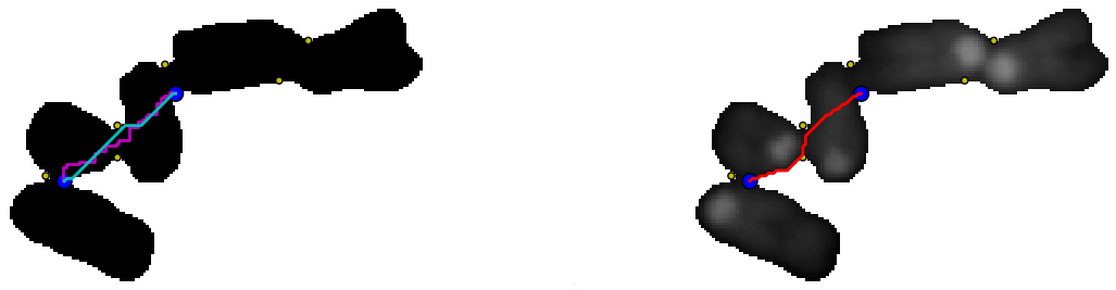
The segmented spots can be overlaid to the original image (blue:telomeric spots, yellow:lines separating the spots after watershed). The quantification can be then performed on the original image (left) but the background must be estimated. The quantification can also be done on the Top-Hat filtered image where the background value is close to zero.

To quantify the spots, two parameters are measured: the spot area and the mean of the spot. The spot intensity is set to the product of the area by the mean gray level value (without taking the exposure time into account).

The area, mean and intensity values can be mapped onto an image or displayed as a histogram (from left to right: histogram of spots mean values, of spots area and histogram of spots intensity).

The following python  script relies on pymorph, mahotas and scipy. It could be tested with skimage.

# -*- coding: utf-8 -*-
"""
Created on Fri Dec 16 13:14:14 2011

@author: Jean-Patrick Pommier
"""

import scipy.ndimage as nd
import pylab as plb
import numpy as np

import mahotas as mh
import pymorph as pm

import skimage as sk
import skimage.morphology as mo

def E_distanceTransform(bIm):
    #from pythonvision.org
    dist = nd.distance_transform_edt(bIm)
    dist = dist.max() - dist
    dist -= dist.min()
    dist = dist/float(dist.ptp()) * 255
    dist = dist.astype(np.uint8)
    return dist
def Chess_distanceTransform(bIm):
    #from pythonvision.org
    dist = nd.distance_transform_cdt(bIm,metric='chessboard')
    dist = dist.max() - dist
    dist -= dist.min()
    dist = dist/float(dist.ptp()) * 255
    dist = dist.astype(np.uint8)
    return dist

def gray12_to8(im):
    i=0.062271062*im
    return pm.to_uint8(i)

path="/home/claire/Applications/ImagesTest/JPP50/16/"
CC="DAPI/"
PR="CY3/" 
im="1.TIF"

dapi=mh.imread(path+CC+im)
cy3=mh.imread(path+PR+im)
#==============================================================================
# Extracting known nuclei
#==============================================================================
nuc=dapi[215:264,1151:1198]
telo=cy3[215:264,1151:1198]
#==============================================================================
# Telomeres Segmentation with pymorph and ndimage
#==============================================================================
op=pm.open(telo,pm.sedisk(5))
top=telo-op
h=pm.hmin(top,200)
remax=pm.regmax(h)
blur=nd.gaussian_filter(h,3)
hi=h-1.0*blur
mask=np.copy(hi)
hi[mask<0]=0
remax=pm.edgeoff(remax)
markers,n=nd.label(remax)
print n," spots detected"
distE=E_distanceTransform(top>200)
distC=Chess_distanceTransform(top>200)
segE,L=pm.cwatershed(distE,markers,return_lines=True)
segC,L=pm.cwatershed(distC,markers,return_lines=True)

#==============================================================================
# Display segmentation on one nucleus
#==============================================================================
print 'display'
RedNuc=mh.bwperim((nuc>1000),n=4)
BlueSpot=mh.bwperim((segE>0),n=4)
GreenSpot=mh.bwperim((segC>0),n=4)


displayTelo=pm.overlay(gray12_to8(telo),red=RedNuc,blue=BlueSpot,yellow=L)
displayTeloC=pm.overlay(gray12_to8(top),red=RedNuc,green=GreenSpot)
#==============================================================================
# Quabtification
#==============================================================================
mean=pm.grain(top,segE,'mean','data')
print np.shape(mean)
area=pm.blob(segE,'area','data')
meanIm=pm.grain(top,segE,'mean','image')
areaIm=pm.blob(segE,'area','image')
print mean
plb.figure(1)
plb.subplot(141,frameon=False, xticks=[], yticks=[])
plb.title('raw 12bits')
plb.imshow(telo)
plb.subplot(142,frameon=False, xticks=[], yticks=[])
plb.title('top Hat')
plb.imshow(top)
plb.subplot(143,frameon=False, xticks=[], yticks=[])
plb.title('hmin')
plb.imshow(h)
plb.subplot(144,frameon=False, xticks=[], yticks=[])
plb.title('regional max')
plb.imshow(remax)

plb.figure(2)
plb.subplot(331,frameon=False, xticks=[], yticks=[])
plb.title('markers')
plb.imshow(markers)
plb.subplot(332,frameon=False, xticks=[], yticks=[])
plb.title('Thresholded Top-Hat')
plb.imshow(top>200)
plb.subplot(334,frameon=False, xticks=[], yticks=[])
plb.title('Euclid dist map ')
plb.imshow(distE)
plb.subplot(335,frameon=False, xticks=[], yticks=[])
plb.title('watershed seg')
plb.imshow(segE)
plb.subplot(333,frameon=False, xticks=[], yticks=[])
plb.title('TopH+hi pass')
plb.imshow(hi)
plb.subplot(337,frameon=False, xticks=[], yticks=[])
plb.title('Chess d map')
plb.imshow(distC)
plb.subplot(338,frameon=False, xticks=[], yticks=[])
plb.title('watershed Chess')
plb.imshow(segC)

plb.figure(3)
plb.subplot(121,frameon=False, xticks=[], yticks=[])
plb.title('telo+seg')
plb.imshow(displayTelo)
plb.subplot(122,frameon=False, xticks=[], yticks=[])
plb.title('telo+seg')
plb.imshow(displayTeloC)

plb.figure(4)
plb.subplot(231,frameon=False, xticks=[], yticks=[])
plb.title('Quant image=mean')
plb.imshow(meanIm)
plb.subplot(232,frameon=False, xticks=[], yticks=[])
plb.title('Quant img=area')
plb.imshow(areaIm)
plb.subplot(233,frameon=False, xticks=[], yticks=[])
plb.title('Quant img=mean*area')
plb.imshow(areaIm*meanIm)
plb.subplot(234)
plb.hist(mean)
plb.subplot(235)
plb.hist(area)
plb.subplot(236)
Q=areaIm*meanIm
plb.hist(Q.flatten()[Q.flatten()>0])
plb.show()

How to rotate faster chromosomes vertically (a little bit)

It is possible to orientate chromosomes vertically with a morphological  "rose des directions" using successive erosions. The larger the particle is, the longer the operation is. However, the iterations can be reduced by submitting not the particle itself, but a Top-Hat version of the image, or the particle skeleton or the particle contour yielding similar results with a reduced cost.

The first rose-des-directions was obtained with the original particle, I didn't compute the total amount of erosion, but finding the principal orientation around 120° required around 50 successive erosions, whereas only 16 erosions are necessary if the particle skeleton is analysed, 30 erosions with the Top-Hat filtered image or 20 with the contour.

With a more complex image, the "rose des directions" detects the orientation of the larger chromosome.

Drag and drop two chromosomes with pygame

Starting to understand how to move sprites with pygame, a small result:

The following code is still not a karyotyper (no classifier). It is a model to understand how to move two sprites.

# -*- coding: utf-8 -*-
"""
@author: jean-pat
"""
#!/usr/bin/env python
#
import os, pygame
from pygame.locals import*

def load_image(name, colorkey=None):
    fullname=os.path.join("data", name)
    try:
        image=pygame.image.load(fullname)
    except pygame.error, message:
        print "Impossible de charger l'image:",name
        raise SystemExit, message
    image = image.convert()
    if colorkey is not None:
        if colorkey is -1:
            colorkey = image.get_at((0, 0))
        image.set_colorkey(colorkey, RLEACCEL)
    return image, image.get_rect()

class Ichrom(pygame.sprite.Sprite):
    def __init__(self,image,initpos):
        pygame.sprite.Sprite.__init__(self)
        self.pos = initpos
        self.image, self.rect=image
        self.button=(0,0,0)#mouse buttons not pressed
        self.selected = 0
        self.mouseover=False
        self.focused=False
        print "init chrom at ",self.pos

    def rollover(self):
        """Test if the mouse fly over the chromosome 
        self.mouseover==True if mouse flying over the chrom,
        False if not"""
        mpos=pygame.mouse.get_pos()#mouseposition
        #test if mouse roll over the sprite
        if self.rect.collidepoint(mpos):
            self.mouseover=True
        else:
            self.mouseover=False
    def update(self):
        self.button=pygame.mouse.get_pressed()
        mpos = pygame.mouse.get_pos()
        self.selected=self.rect.collidepoint(mpos)
        #the mouse flies over a chromosome
        if (self.mouseover):
            #print "mouse pos:",mpos
            if self.button==(1,0,0):     # )  
                pos = pygame.mouse.get_pos()
                self.rect.midtop = pos

def main():
    pygame.init()
    screen = pygame.display.set_mode((400,300))
    pygame.display.set_caption("Karyotyper")
    pygame.mouse.set_visible(True)
    
    background = pygame.Surface(screen.get_size())
    background = background.convert()
    background.fill((0, 0, 0))

    screen.blit(background,(0, 0))
    pygame.display.flip()
    
    i1=load_image("/home/claire/Applications/ImagesTest/jp/Jpp48/13/DAPI/particules/part15.png", -1)
    i2=load_image("/home/claire/Applications/ImagesTest/jp/Jpp48/13/DAPI/particules/part9.png", -1)
    chr1 = Ichrom(i1,(0,0))
    chr2=Ichrom(i2,(30,30))
    allsprites = pygame.sprite.RenderPlain((chr1,chr2))
    clock = pygame.time.Clock()

    while 1:
        clock.tick(60)
        for event in pygame.event.get():
            if event.type == QUIT:
                return
            elif event.type == KEYDOWN and event.key == K_ESCAPE:
                return
            if event.type ==pygame.MOUSEBUTTONDOWN:
                #need to be modified to handle a list of chromosomes
                chr1.rollover()
                chr2.rollover()
        allsprites.update()
        screen.blit(background,(0,0))
        allsprites.draw(screen)
        pygame.display.flip()
    
if __name__ == '__main__': main()

Highlighting Interstitial Telomeric Spots in interphasic cells (HITS-FISH)

Telomeric fusions underscore telomeric binding proteins disfunctions. Fusions occur in senescent cells between short telomeres, they are detected in metaphasic cells by dicentric chromosomes most generally with no telomeric spots at the fusion point.

In some SV40 transformed fibroblast cell line, interstitial telomeric spots (ITS) are as bright as terminal telomeric spots, this indicates some uncoupling between telomere lenght and their capacity to block telomeric fusions. 

ITS observed in a precrisis human SV40 transformed cell line (Ducray et al., oncogene 1999)

From metaphasic chromosomes observation, fusions retaining visible telomeric spots are rare events but may be more frequent in interphasic cells.

ITS from a SV40 transformed cell line

Bal31 in-situ:

Several nucleases or DNA polymerases  were used in assays requiring fixed material (chromosome banding+restriction endonuclease, in-situ nick translation, fluorescent labelling with TUNEL, in-situ PCR). The exonuclease Bal31 removes totally terminal telomeric sequences of naked DNA after some hours of digestion (R C Allshire, M Dempster, and N D Hastie, NAR 1989; de Lange et al, MCB 1990) . In-situ,  the terminal telomeric sequences, should be removed by Bal31 digestion.  If telomeric spots can be detected in nuclei after Bal31 digestion, those spots should be  ITS. Monitoring ITS may be a tool of interest  to probe telesome functions at the scale of unique cell, or to monitor the state of a tissue.

Pig cells as model cells?

On human metaphasic chromosomes, a bright ITS indicates an  abnormal cell but for cheaper DAPI stained chromosomes rearrangements too. Normal pig karyotype  shows interstitial telomeric spots:

Normal diploid pig metaphase with a chromosomes pair having ITS.

After QFISH on interphasic pig nuclei, there are two ITS of same magnitude than terminal spots, these two pig ITS remain hidden in the forest of terminal telomeric spots:

  

Pig nuclei (25x magnification)

Some conditions of Bal31 digestion should retain these two ITS and remove totally terminal telomeric spots yielding the possibility to observe telomeric fusions in nuclei.

Assay:

Tuning the conditions of Bal31 digestion is a prerequisite step. Supposing that the exonuclease Bal31 can remove terminal sequence from fixed material, when this enzyme is usually used to digest purified DNA in solution. 

If pig cells are not available, performing Bal31 digestion on control human cells such lymphocytes should tell if Bal31 can remove telomeres in-situ.

From conventionnal cytogenetic preparation of pig cells (fibroblasts,lymphocytes), digestion time, numbers of Bal31 units could be set up as follow : 

Possible protocol for HITS FISH

The protocol modified from Lansdorp et al. (Hum Mol Genet. 1996 May;5(5):685-91.) could be also adapted to liquid hybridization for flow FISH. Under optimal conditions pig cells could be used as internal control for Bal 31 digestion by mixing human and pig cells in the same cytogenetic preparation (9:1 ratio).

Human cells can be then distinguished from pig cells with an additionnal oligo probe. In the following example (25x magnification), simultaneous hybridization with Cy3-PNA-(CCCTAA)3 (displayed in green) and Cy5-DNA (displayed in red) oligo probe was performed (unpublished data):

Candidate cells to test the assay, may be SV40 precrisis cells with highly rearranged chromosomes and numerous dicentrics, or better cells with controlled mutations.

Particle : a python class to compute particle anisotropy by morphological erosion

A python class called particle, is implemented to handle the chromosomes extracted from a metaphase image:

Original segmented chromosomes

The class particle  is instanciated with the counterstain image (DAPI), it is possible to :

1. display a particle vertically
2. compute the convex hull area. The convex hull area is computed with from the coordinates of the convex hull vertices.
3. produce the morphological rose des directions, which describe the particle anisotropy.

Blue curve:orientation curve (rose des direction) for the original particle image (top left). Green curve: orientation curve after high pass filtering (top right).

The script written to test the class, instanciates two particle objects, for example:

•  p1=particle(im), where im is a DAPI image of segmented chromosomes.

It is then possible to get the morphological "rose des directions", that is the number of morphological erosion by a 1x3 structuring element, necessary to erode totally the particle in a given direction:

• theta1,rosedirections,VImage=p1.orientationByErosion(10) 

• The parameter set to 10 is the rotation step
• theta: the particle principal orientation
• rosedirections: a numpy array to plot the erosion number vs the rotation angle
• VImage: rotated particle image

 The particle convex hull is obtained with:

• p1.cvxhull_area()

The script must be modified to fit  the image path.

Numpy, scipy, matplotlib, pymorph, readmagick, mahotas must be installed. However since original implementation. Mahotas itself or scikit image could be used instead of readmagick to load the image.

With two features, as the particle area and the ratio between the particle area and the convex hull area, it should be possible to start to classify the particles into four categories:

• non overlapping chromosomes,
• overlapping chromosomes,
• nuclei, 
• remaining small stuffs .

Code on Gist 

anisotropy_RoseDirections.py

Ipython notebook here

http://nbviewer.ipython.org/gist/jeanpat/7673858 

Metaphase chromosomes segmentation with ImageJ

Chromosomes segmentation is the first step of MFISH or QFISH analysis.

Let's try to identify chromosomes from a DAPI stained metaphase:

The image was  acquired with a 12 bits CCD camera. Microscopic field illumination is supposed homogeneous and no flat-field correction will be performed.

To segment the chromosomes, first check that Gabriel Landini's morpholological plugins is installed, and  load the image with ImageJ. ImageJ indicates that the image is now a 16 bits image. 

The interphasic nuclei yield saturated pixels at 4095 in the image histogram :

The gray level value of the first peak corresponding to the backgroung is around 300. Let's substract this value to the image and then perform a local background substraction with a rolling ball value set to 15 using the Hilo LUT to visualize the background.

Now the image histogram yields:

Erase the pieces of nuclei with the eraser tool. Threshold the image interactively and label the binary image then display it with the 3-3-3 RGB LUT:

This procedure yields under segmented chromosomes. From the original binary image. By performing a watershed and relabel the new image, we get:

The touching chromosomes are now well separated but most chromosomes are now over segmented, anyway the result may be interesting since the parts obtained grossly corresponds to p and q chromosomal arms.

To get a good segmentation, an interactive step with the drawing tool may be here necessary:

Another example of chromosomes segmentation without manual modification (that is without painting tools) leading to over segmentation:

Here identifying first the chromosomes help to choose parameters to perform chromosomes segmentation. Some iterations between image segmentation and the chromosomes recognition step must be introduced to automatise the process.