Telomeres quantification in a nucleus

Telomeres quantification can be done at low magnification in interphasic cells. A microscopic field was recorded with a CCD camera at low magnification (objective x25). Nuclei were counterstained with DAPI and the telomeres were detected with a Cy3-PNA probe.

From the field image, a nucleus is segmented and the DAPI and Cy3 spectral components are isolated. Even at low magnification, the telomeric spots can be segmented as follow:

Background is removed by top-hat filtering with a small structuring element (a disk of size=5). The top-hat image is then submitted to a hmin operator, leaving the peaks higher than 200 gray level units, then regional maxima are found.

The regional maxima are labelled to obtain markers for the watershed algorithm. Once thresholded, the top hat image is converted into distance map using euclidian or chess-board distance without significant difference.

Watershed doesn't succeed very well in separating spots belonging to the lower cluster of three spots. It may be interesting to use a high pass filtered image to build a  distance map.

The segmented spots can be overlaid to the original image (blue:telomeric spots, yellow:lines separating the spots after watershed). The quantification can be then performed on the original image (left) but the background must be estimated. The quantification can also be done on the Top-Hat filtered image where the background value is close to zero.

To quantify the spots, two parameters are measured: the spot area and the mean of the spot. The spot intensity is set to the product of the area by the mean gray level value (without taking the exposure time into account).

The area, mean and intensity values can be mapped onto an image or displayed as a histogram (from left to right: histogram of spots mean values, of spots area and histogram of spots intensity).

The following python  script relies on pymorph, mahotas and scipy. It could be tested with skimage.

# -*- coding: utf-8 -*-
"""
Created on Fri Dec 16 13:14:14 2011

@author: Jean-Patrick Pommier
"""

import scipy.ndimage as nd
import pylab as plb
import numpy as np

import mahotas as mh
import pymorph as pm

import skimage as sk
import skimage.morphology as mo

def E_distanceTransform(bIm):
    #from pythonvision.org
    dist = nd.distance_transform_edt(bIm)
    dist = dist.max() - dist
    dist -= dist.min()
    dist = dist/float(dist.ptp()) * 255
    dist = dist.astype(np.uint8)
    return dist
def Chess_distanceTransform(bIm):
    #from pythonvision.org
    dist = nd.distance_transform_cdt(bIm,metric='chessboard')
    dist = dist.max() - dist
    dist -= dist.min()
    dist = dist/float(dist.ptp()) * 255
    dist = dist.astype(np.uint8)
    return dist

def gray12_to8(im):
    i=0.062271062*im
    return pm.to_uint8(i)

path="/home/claire/Applications/ImagesTest/JPP50/16/"
CC="DAPI/"
PR="CY3/" 
im="1.TIF"

dapi=mh.imread(path+CC+im)
cy3=mh.imread(path+PR+im)
#==============================================================================
# Extracting known nuclei
#==============================================================================
nuc=dapi[215:264,1151:1198]
telo=cy3[215:264,1151:1198]
#==============================================================================
# Telomeres Segmentation with pymorph and ndimage
#==============================================================================
op=pm.open(telo,pm.sedisk(5))
top=telo-op
h=pm.hmin(top,200)
remax=pm.regmax(h)
blur=nd.gaussian_filter(h,3)
hi=h-1.0*blur
mask=np.copy(hi)
hi[mask<0]=0
remax=pm.edgeoff(remax)
markers,n=nd.label(remax)
print n," spots detected"
distE=E_distanceTransform(top>200)
distC=Chess_distanceTransform(top>200)
segE,L=pm.cwatershed(distE,markers,return_lines=True)
segC,L=pm.cwatershed(distC,markers,return_lines=True)

#==============================================================================
# Display segmentation on one nucleus
#==============================================================================
print 'display'
RedNuc=mh.bwperim((nuc>1000),n=4)
BlueSpot=mh.bwperim((segE>0),n=4)
GreenSpot=mh.bwperim((segC>0),n=4)


displayTelo=pm.overlay(gray12_to8(telo),red=RedNuc,blue=BlueSpot,yellow=L)
displayTeloC=pm.overlay(gray12_to8(top),red=RedNuc,green=GreenSpot)
#==============================================================================
# Quabtification
#==============================================================================
mean=pm.grain(top,segE,'mean','data')
print np.shape(mean)
area=pm.blob(segE,'area','data')
meanIm=pm.grain(top,segE,'mean','image')
areaIm=pm.blob(segE,'area','image')
print mean
plb.figure(1)
plb.subplot(141,frameon=False, xticks=[], yticks=[])
plb.title('raw 12bits')
plb.imshow(telo)
plb.subplot(142,frameon=False, xticks=[], yticks=[])
plb.title('top Hat')
plb.imshow(top)
plb.subplot(143,frameon=False, xticks=[], yticks=[])
plb.title('hmin')
plb.imshow(h)
plb.subplot(144,frameon=False, xticks=[], yticks=[])
plb.title('regional max')
plb.imshow(remax)

plb.figure(2)
plb.subplot(331,frameon=False, xticks=[], yticks=[])
plb.title('markers')
plb.imshow(markers)
plb.subplot(332,frameon=False, xticks=[], yticks=[])
plb.title('Thresholded Top-Hat')
plb.imshow(top>200)
plb.subplot(334,frameon=False, xticks=[], yticks=[])
plb.title('Euclid dist map ')
plb.imshow(distE)
plb.subplot(335,frameon=False, xticks=[], yticks=[])
plb.title('watershed seg')
plb.imshow(segE)
plb.subplot(333,frameon=False, xticks=[], yticks=[])
plb.title('TopH+hi pass')
plb.imshow(hi)
plb.subplot(337,frameon=False, xticks=[], yticks=[])
plb.title('Chess d map')
plb.imshow(distC)
plb.subplot(338,frameon=False, xticks=[], yticks=[])
plb.title('watershed Chess')
plb.imshow(segC)

plb.figure(3)
plb.subplot(121,frameon=False, xticks=[], yticks=[])
plb.title('telo+seg')
plb.imshow(displayTelo)
plb.subplot(122,frameon=False, xticks=[], yticks=[])
plb.title('telo+seg')
plb.imshow(displayTeloC)

plb.figure(4)
plb.subplot(231,frameon=False, xticks=[], yticks=[])
plb.title('Quant image=mean')
plb.imshow(meanIm)
plb.subplot(232,frameon=False, xticks=[], yticks=[])
plb.title('Quant img=area')
plb.imshow(areaIm)
plb.subplot(233,frameon=False, xticks=[], yticks=[])
plb.title('Quant img=mean*area')
plb.imshow(areaIm*meanIm)
plb.subplot(234)
plb.hist(mean)
plb.subplot(235)
plb.hist(area)
plb.subplot(236)
Q=areaIm*meanIm
plb.hist(Q.flatten()[Q.flatten()>0])
plb.show()

Toward robust chromatids labelling :

Holed, bended, round shaped chromosomes may lead to poor chromatids labelling with one pair of gray seeds. Here with several pairs of seeds, a much better labelling is reached:

 

Chromatids labelling after watershed

 The result depends on how the seeds were chosen. Four independent factors must be taken into account:

• The pairs of seeds number:
• One pair yields poor results as observed previously.
• The orientation of the pair of seeds  relative to the chromosome
• The axis of the pair of seeds, must be locally orthogonal to the axis of the chromosome.
• For a given pair of seeds, the distance between the two discs.
• The relative orientation of the pair of seeds
• The pair of seeds must have the same orientation

The seeds used to get the result were choosen by hand:

seeds and edge of binary chromosomes in false colors.

When the seeds don't have the same orientation, watershed yields an harlequin  pattern :

Harlequin pattern (black holes are due to the absence of seeds to label the background)

Labelling chromosome-like shapes using watershed: effect of the chromosome shape

[edit feb 2013]
In previous post, the  chromatids of metaphasic chromosomes were labelled by hand with a painting tool in ImageJ following a watershed segmentation step:

Initial chromatids segmentation in ImageJ after high pass  filtering, thresholding, watershed and image labelling.

Final chromatids (blue or green) segmentation after painting by hand, centromeric region was added and paint in red.

 With a simplistic rigid model of chromosome and well chosen seeds, a watershed can label the chromatids:

Chromosomes present variable shapes, metacentric chromosomes are X shaped, acrocentric chromosomes are Y-shaped. The  shape of the same chromosome varies also from one metaphase spread to another, it can be randomly bended,condensed. Image processing introduces also variability according to the parameters used (threshold, filtering ...). Is it possible to segment chromatids such conditions ? Let submit a contour image of chromosome-like shapes to wateshed algorithm implemented in mahotas:

model shapes of chromosomes of variable size, bending. (Gimp)

seeds: the darkest seeds will label the back ground, they are outside the chromosomes. The pairs of lighter seeds are supposed to label the chromatids. (The Gimp)

In a python console:

    PyShell 0.9.8 - The Flakiest Python Shell
    Python 2.6.6 (r266:84292, Sep 15 2010, 15:52:39)
    [GCC 4.4.5] on linux2
    Type "help", "copyright", "credits" or "license" for more information.
    Startup script executed: /home/claire/.pyshell/startup
   >>> g=readmagick.readimg("/home/claire/Applications/ImagesTest/essai02/grad.tif")
   >>> s=readmagick.readimg("/home/claire/Applications/ImagesTest/essai02/seeds.tif")
   >>> label=mahotas.cwatershed(g, s, Bc=None, return_lines=False)
   >>> readmagick.writeimg(label,"/home/claire/Applications/ImagesTest/essai02/label.tif")

The background is labelled with one seeds outside the chromosomes and with seeds (same grey level) inside the chromosome holes. The chromatids are labelled with one pair of seeds inside the chromosomes:

Pair of seeds for watershed with two different grey levels

They are chosen grossly to fall apart the chromosomal axe:

Labelling with one pair of seeds per chromosome

If several pair of seeds are chosen by hand, a better chromatid segmentation can be found:

Pair of seeds overlaid to the particles contour

Chromatids like segmentation

The result depends on how the seeds were chosen. Four independent factors seems to be considered:

• Seeds number:  one pair yields poor results as observed previously.
• Seeds orientation : the seeds axis, must be locally orthogonal to the axis of the chromosome.
• For a given pair of seeds, the distance between the two discs.
• Relative orientation of the pair of seeds: The pair of seeds must have the same orientation.

When the seeds don't have the same relative orientation, watershed yields an harlequin  pattern :

opposite pair of seed yield harlequin pattern

Up to now, image labelling was performed with seeds chosen manually and drawn by hand with the gimp or ImageJ. The seeds localization have to be found automatically and mathematical morphology may provide solutions. The chromosomal axis is close to the particle skeleton. Can the particle skeleton be used to automatically find seeds useful for chromatid labelling with watershed? Using ImageJ interactively, chromosome-like particles skeleton was found:

chromosome-like particles

particles skeletons

From the skeleton, the branching points and end-points are searched using a binary hit-or-miss operator in ImageJ (see here for code). Different hit-or-miss structuring elements suceed in detecting branching points. If end-points and branching points are overlaid on the binary particules, chromosomal areas close to those chosen by hand, are finally found:

Skeleton branching points (color), skeleton end points (black)

At first sight end-points would provide better candidate seeds for watershed.

Good seeds, bad seeds :using watershed to label chromatids of a metacentric model chromosome

A model image of a metacentric chromosome was generated with ImageJ. The model is simplistic, it consists in X shaped binary image:

16 bits binary  image

The seeds consists in small spots in a image. To detect the chromatids, the seeds are designed as two discs labelled by two different gray level (one for each chromatid).

The initial location of the seeds, was in that first trial choosen by hand.

Initial seeds location inside the chromosome 

Gray seeds (that is a 16 bits grayscale image) are then allowed to grow using the watershed algorithm inside the chromosomes, yielding(the result is displayed with pylab):

seeds after watershed yield labelled chromatids (light blue, dark blue)

The result is nice because the initial location was purposefully chosen. What would happen with varying seeds location or orientation ?

Seeds location shifted in the lower left chromatid

After rotation, the seeds can label  p and q arms:

Upper left: the seeds are 45° rotated, the p arm (light blue) and the q arm (dark blue) are detected.

Upper, lower right: shifting vertically the seeds 

Lower left:use of three seeds p  arm (blue), centromeric region (green), q arm (yellow)

Chromatids segmentation with ImageJ

Let's perform high pass filtering on the DAPI image previously processed:

After thresholding and connected component labeling, we get:

If prior image labelling, watershed is performed, the chromosomes are broken into particles that corresponds mainly to the chromatids of the largest chromosomes:

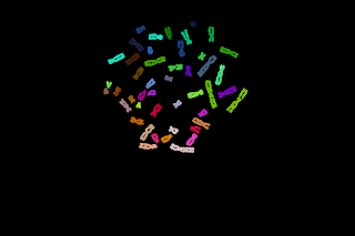
We can see that most of the chromatids are well detected in large chromosomes but less accurately in small chomosomes such HSA 19 or HSA21:

Some pieces of chromatids are well detected, let's paint ("Human labeling") them by hand:

• in green or blue for the chromatids 
• in red for the centromeric labeling
• in yellow, for the badly segmented chromatids.

Yellow regions needs to be reaffected to blue / green or red region. By hands, it gives:

Can we imagine an algorithm capable to perform that task?
A low level image opening finally yields: