Construct a graph from the skeleton image of a binary form

Previously an attempt was made to write a code capable of building a graph from the skeleton of an image and it was not a complete success since some preprocessing (pruning) had to be done to build a graph. Here an other python code was written and at very first sight, it seems to produce a graph without complaining....sometimes (see at the end).

The code was run in a ipython notebook running on sagemath cloud. It relies on several libraries : mahotas and networkx, numpy is provided by default. Scikit image was also tested. Pillow was used to generate images of some letter as model.

The idea is the following:

• make the skeleton of a binary image.
• get its branched-points and add them in a graph.
• get its end-points, add them to the graph.
• get the edges of the skeleton and decompose them into:
• edges between end-points and branched-points.
• edges between branched points.
• add edges to the graph between end-points and branched-points.
• add edges to the graph between branched-points.

Images models

Since the code is run on sagemath cloud, Pillow has to be installed. From a terminal :

pip install Pillow

 The verdana true type font was obtained from fontsupply and the file verdana.ttf had to be at the same location than the ipython notebook ( verdana.ttf was uploaded on SMC project at the same location than the ipython notebook).

The code used to generate images and draw them is:

and we get:

What kind of skeleton?

Both mahotas an scikit-image implement morphological operators to generate the skeleton of a binary shape. Scikit-image seems to use a neighbourhood  on 4 pixels (C4) and mahotas on on neighbourhood of 8 pixels (C8). This is why mahotas was retained to produce skeletons:

• medial axis  of the letter A computed with scikit image (left), branched points and end-points are extracted using hit-or-miss operator implemented in mahotas (middle). The branched-points can be removed from the medial axis and the resulting image can be labelled (left), pixels connected only vertically or horizontally share the same label.

Skeleton from the letter A (left)

•  If a skeleton is generated by morphological thining with mahotas, we get the left image. The fourth image is the skeleton deprived of its branched points. Scikit-image provide a thining operator with a C4 neighborhood (right image):

 

C8 skeleton by thining (left). C4 skeleton by thining (right).

What's happen if a C8 skeleton is labeled? Here, both mahotas and scikit-image provide the same result:

edges (mahotas:left; scikit-image:right)

The labelled regions fit here what can be seen as an edges.

Prior to start to build a graph, several additionnal images are needed:

Edges decomposition:

Let's decompose the image of edges by considering edges connecting end-points to branched-points and edges connecting only branched points:

Starting to build the graph by the branched-points:

 The branched-points are added first. The branched point of label 1 in the image, is the first vertex in the graph, and so on:

The end points are the added to the graph, there is a shift between the end-points label in the image and their index in the graph. The first end-point in the image will be the fith vertex in the graph:

The vertex of the graph (G) have attributes derived from the images they come from: their position 'pos' define by (row,col), their label in the image of origin. Typing in a ipython cell:

          print G.nodes(data=True)
          print nx.get_node_attributes(G,'label')

yields:

[(1, {'pos': (3, 9), 'label': 1}), (2, {'pos': (3, 12), 'label': 2}), (3, {'pos': (17, 5), 'label': 3}), (4, {'pos': (17, 17), 'label': 4}), (5, {'pos': (1, 9), 'label': 1}), (6, {'pos': (1, 13), 'label': 2}), (7, {'pos': (25, 3), 'label': 6}), (8, {'pos': (25, 21), 'label': 8})]
{1: 1, 2: 2, 3: 3, 4: 4, 5: 1, 6: 2, 7: 6, 8: 8}

Linking end-points to branched points:

 The idea here is to get the neighbourhood of each branched-point in the "edges ep-ep" image and to add an edge in the graph between the corresponding branch-point and end-point(s). This yield:

Linking branched-points

•  A dictionnary where the keys are the labels of the branched-points and the values are the label of the "edges bp-bp" in the neighbourhood of the branched point is build. Thus there's one key (bp label) for several values (edges labels).
• But an edge can be seen as one key (the edge label) for two values (the two labels of the two branched-points). So the dictionnary has to be inverted in that very particular way. Fortunately, that problem was solved on stackoverflow.

 Finaly, we have:

 the whole steps are gathered in a function:

Processing other  letters gives for example:

The ipython notebook is here:

View the notebook on ipython.org

Sometimes building the graph fails:

On a larger set of images:

• For the image corresponding to the letter K, the graph construction fails due to the presence of branched regions made of several pixels instead of one.
• There's also a problem with the letter D, its graph has no loop.
• Since there's no branched point in the skeleton of the letter C, its graph is not build.

 The ipython notebook has been reordered and is available on ipython.org

An endpoints spectrum:possible features from the skeleton?

Looking for topological features:

The skeleton of a binary shape can be used to find features to classify it. The number of endpoints or the number of branched points should be good candidates. A shape which skeleton has no endpoint nor no branched point could be a circle:

 O

A shape with one branched point and no endpoint, may looks like this :

8

Binary model shapes were loaded in an ipython notebook with skimage which was capable of handling .pgm format :

Skeletons were generated by morphological thinning implemented in  mahotas:

endpoints (blue), branched points (green)

Endpoints Spectrum :

The skeleton of the hand has two endpoints close to top of each fingers, as it would be fine to have one endpoint per finger, let's prune the skeleton to meet this condition. This can be achieved after some trial, however if robust features could be found from the skeleton a systematic method is needed. So, let's prune the skeleton until it has no endpoint and count the number of pruning step necessary:

From the curve, the hand skeleton has 13 endpoints before any pruning, after 40 pruning steps, it has 6 endpoints. Around 90 pruning steps are necessary to remove all endpoints. By only looking at their curve, the hand shaped silhouette and the fish shaped silhouette are different.

Endpoints spectrum resists to scale variation after normalization:

As scale invariance is a nice feature, let's see what is happening when the scale of the shape is successively reduced by a factor of 0.9², 0.7², 0.5², 0.3²:

From the images above, it is clear that  the skeleton resists to scale variations but as the skeleton becomes smaller  less pruning steps are necessary to "burn" it to the last pruned pixels set. So let's norme the pruning steps by the initial skeleton size such for 0 pruning step, the normed pruning step is 100. As the size of the hand shaped silhouette decreases (from 81%, 49%, 25%, 9% of the original size), the endpoints spectrums  remain comparable:

Endpoints spectrum of similar shapes are similar:

How does the curve behave with similar shapes? Let's compare the endpoints spectrum of the serie of six hands:

The spectrums seem to resist to shape rotation (hand, hand-10°, hand90°) and to moderate shape deformation (hand-bent1,2). The sketch-hand silhouette is a right hand and its spectrum is comparable to the other spectrums which corresponds to left hands, so the endpoints spectrum is symetry invariant too.

Deriving a features vector from endpoints spectrum:

If shapes should be classified according to their topology, the whole endpoints spectrum is not necessary and only the transitions may be retained. Taking a  hypothetical skeleton whose endpoints spectrum before normalization is:

• For 7 prunings the skeleton has 0 endpoints

•       6                                        1

•       2                                        3

•       0                                        4

So a possible features vector would be:

(7,6,-1,2,0)

The value -1 indicates that the value 2 endpoints is missing. In the python script, the endpoints spectrum is coded as two lists:
             end_points_test   = [4,3,3,1,1,1,1,0]
             pruning_steps_test = [0,1,2,3,4,5,6,7]
A python function taking the steps list and the endpoints (spectrum) list yields a features vector :

def EPSpectrumToFeatures(steps, spectrum):
    '''
          eptest   = [4,3,3,1,1,1,1,0]
          pruntest = [0,1,2,3,4,5,6,7]
the returned vec:[7,6,-1,2,0] which means:
    0 enpoints -> 7 prunings necessary
    1 endpoint -> 6 prunings
    4 endpoints-> 0 pruning (initial skeleton size)
'''
     values = set(spectrum)
    feat_vect = [-1]*(len(values)+1)
    spec = np.asarray(spectrum)
    for epn in values:
        indexmin = np.where(spec == epn)[0][-1]
        feat_vect[epn] = steps[indexmin]
    return feat_vect
Supposing now the the skeleton size is 25, let's normalise the pruning steps as follow: 

 normed_pruning_steps_test = [100*(1-i/25.0) for i in pruntest] 

The endpoints spectrum is:

Let's take a normalised endpoints spectrum:

• normedsteps = [100.0, 96.0, 92.0, 88.0, 84.0, 80.0, 76.0, 72.0]

• endpoints = [4, 3, 3, 1, 1, 1, 1, 0] 

And let's submit it the previous function :

EPSpectrumToFeatures(normedsteps, endpoints)

 The function yields the vector:

[72.0, 76.0, -1, 92.0, 100.0]

which means that the skeleton has:

• 0 endpoint for a normed number of  prunings of 72%
• 1  ---------------------------------------------------------------------------76%
• no 2 endpoints, set normed number of  prunings to -1
• 3 -------------------------------------------------------------------- 92%
• 4 ------------------------------------------------------------------ 100%

The different endpoints spectrum curves suggest that the vector could used for classifying 2D binary shapes.

A feature vector from a real shape:

Let's consider the shape of a hand:

Its endpoints spectrum (normalised by skeleton size or not) was calculated and a feature vector was derived and displayed (red) with the spectrum:

Left: raw endpoints spectrum (blue) and its feature vector (red). Right: Normed endpoints spectrum and its feature vector, for 100% of the skeleton size, the skeleton has 14 endpoints, for ~94% the skeleton has 7 endpoints and for 83% of the skeleton size the skeleton has no endpoint.

For a larger number of image a python class, called Shape was written. It is instantiated as follow: 

shape= Shape(image)

The feature vector can be computed by:

vector = shape.End_Points_Features(normed = True)

or by:

vector = shape.End_Points_Features(normed = False)

Feature vectors from 216 images :

216 images of small 2D binary images (silhouettes) [Sharvit et al.] were used to derive feature vectors. This set of images consists in 18 type of silhouettes with 12 instance of each. For example, there are 12 birds silhouettes:

Prior any kind of classification the 216 normed feature vectors were aligned for visual inspection:

Some silhouettes, as the Bone silhouettes seems to show some intra-class structure, while Brick and Camel silhouettes seems different.

ipython notebook (updated 24/05/2013):

All the  tasks were performed in a ipython notebook available here.

 

Trying to separate touching mouse chromosomes

In the previous post, from a cluster of touching mouse chromosomes:

points belonging to negatively curved domains of a contour can be isolated :

Yellow points belong to negatively curved domains of the contour.

To separate the chromosomes, it is tempting to cut between the closest pairs of points.

Let's make combination of pairs of points belonging to the contour:

Python provides itertools.combinations(); the closest pairs of points are in the set of the combinations of every pairs of points:

Path between two points belonging to the countour:

Each line shows the euclidian distance between two points, the four shortest lines correspond more or less to the contact domains between the chromosomes, cuting along them provides a way to separate the chromosomes.

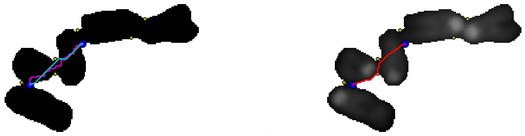
It should be possible to do better by using a geodesic distance between the points, that is using a path inside the cluster of chromosomes. In the following example:

On the left, two paths (depending on the chosen pixel neighborhood) between the two blue points were overlaid on a binary image (background is set to 255 and the foreground to 0). The path were determined as follow using skimage 0.8dev:

graph.route_through_array(negbin ,p1,p2,fully_connected=False)

 or

 graph.route_through_array(negbin ,p1,p2,fully_connected=True)

• negbin: the negative binary image
• p1, p2: the two points figured in blue.

On the right the background (0) was set to 255 (white), the path (red) between the two points was determined by minimizing the "greyscale cost", that is through the valleys between the two points is the image is viewed as a greyscaled landscape.

All the paths can be determined (left), and then the paths can be sorted according to their cost (right). The four paths with the smallest cost are figured in red (left).

Download code.

or see bellow:

Contour : looking for negatively curved domains

A contour was previously explored with the convexity defects  algorithm implemented in opencv. Some highly curved domains  failed to be detected because of the contour shape.

Curved domains missed by convexity defects detection

Using polygonal approximation imlemented in skimage 0.8 dev, positively curved domains as well as negatively curved domains on a contour can be sorted:

Contour of a chromosomes cluster (blue), polygonal approximation (yellow). Red points: positive curvature. Yellow points: negative curvature.

From a segmented particle, a polygonal approximation of the contour is extracted.

Points of the polygon are used to compute an angle between two consecutive vectors (Here using the complex affix of vectors):

Positive angles correspond to convex domains and negative angles to concave domains.

The code has to be modified to filter angles according to a given range. 

The code can be modified as follow to filter angles corresponding to curved domains:

• positive = table[(135>table[:,2]) & (table[:,2]>45)]

• negative = table[(-45>table[:,2]) & (table[:,2]>-135)]

Curved domains on polygonal approximation of a chromosomes cluster contour.

Download code

Touching chromosomes, overlapping chromosomes, single chromosomes and their convexity defects

Let's start with convexity defects (blue circles) detected in totally overlapping chromosomes:

The convexity defects can be directly used to resolve the two overlapping chromosomes, the script is used with d>1000 (see the two previous posts).

When the chromosomes partially overlap, we can have less than four points detected:

As in the previous post, touching chromosomes produce convexity defects. In the following example of two small chromosomes, the two convexity defects detected surrounds the "touching region" . Tracing a segment between the two points would cut the particle (green contour) into two complete chromosomes.

 However touching chromosomes do not always produce  "good" pair of convexity defects which could be used to separate them. In the two following examples, we have two kinds of convexity defects (CD): CDs closed to the touching domain (at coordinates:grossly [30;20] or [40;75] )and CDs near the  centromere (coordinates [35;60]).

Two CDs near the centromere, one CD near the touching region.

Two CDs around the touching region, one CD near the centromere

 In the following cluster of four human chromosomes, only CDs corresponding to the three touching domains were detected. Note that a point at (50,80) corresponding to a touching domain in a highly bended part of the contour and quit far from the convex hull (red) was not detected:

Convexity defects are also detected on single chromosomes keeping the same parameters (d>1000). Let's start with two good cases where the pair of CDs are around the centromere:

The chromosome morphology can alter the detection:

In all the previous example, only CDs with d>1000 were kept. Lowering the  threshold for the d value increases the number of CDs, here is some examples with single chromosomes:

Probably HSA2 chromosome: d>100 : Two CDs are close to the centromere, the others are false positive CD

d>500 : one false positive CD for centromere detection

d>1000 : only one CD near the centromere is detected

For a smaller chromosome (may be chromosome 17), we get:

CD with d>1000

CD with d>500