Showing posts with label chromosomes. Show all posts

Wednesday, July 7, 2021

Back to COCO 2: A less minimalistic 125 images +json dataset

125 grey scaled images were chosen from a previous dataset available on github.

An annotation file was generated by hand online with makesense.ai and saved as a unique json file in COCO format. This small dataset is freely available as an archive.

Check annotation file validity with pycococreator.

Pycococreator by Waspinator was used to display the annotations  (aka the segmentation) over a grey scaled image in the following jupyter notebook 


validating de facto the annotation file produced with makesense.ai:


Data registration in detectron2:

This  is the next step.

The idea is to follow the tutorial on custom dataset registration, possibly using the balloons example by davamix.


Tuesday, May 2, 2017

Resolution of pairs of overlapping chromosomes by semantic segmentation: results from cooperation.

Recently, Rohit Gosh and  Lily Hu  posted reports that a neural network called U-Net can be trained to resolve pairs of overlapping chromosomes.

The story of the dataset:

A first version of the dataset was proposed on kaggle:
By that time, François Chollet, the developper of Keras, openned the ai.on project, a place where to propose different problems to be takled with artificial intelligence approaches.
The "chromosomes problem" was retained and a community of interrested peoples started to think on the problem (There's also a google group)

First results

Rohit Ghosh tried to mix both categories of pixels belonging to non overlapping chromosomes (green), this results in 97% accuracy in the predicted mask !! However, this can lead to combinatoric issues when trying to solve the overlapp.

Rohit Ghosh's results considering overlapping pixels and mixing single chromsomes in a unique class of pixels.

Rohit Ghosh succeeded also in training a U-Net to predict the three labels:

Rohit Ghosh's results on training U-Net to predict the three labels.

According to Rohit Ghosh, when the three labels are predicted, the prediction can reach an accuracy above 80%.

Lily Hu's results

Lily Hu succeeded to train a modified version of U-net (It again !), here's what she got:

Examples of Lily's Hu results (https://blog.insightdatascience.com/separating-overlapping-chromosomes-with-deep-learning-based-image-segmentation-22f97afd3283)

Here the single chromosomes are are represented in red/green and the overlapping domain in blue. All the examples represents,partial overlapps (the cytogeneticist's nightmare). The second prediction is a little bit weird, but the remaining are  really good.
As mentionned in her post, Lily Hu had to pre-process the labels to remove spurious pixels:
https://blog.insightdatascience.com/separating-overlapping-chromosomes-with-deep-learning-based-image-segmentation-22f97afd3283

I am totally guilty, those pixels originate from the fact that masks were generated prior chromosomes rotation as it was explained:

Example of chromosome resolution (with removing of spurious pixels)

In the new version dataset, the labels are clean.

The traing curves are interresting:
https://blog.insightdatascience.com/separating-overlapping-chromosomes-with-deep-learning-based-image-segmentation-22f97afd3283

 The IOU index for overlapping pixels is above 90%!! Wow!

I suspect that with the new generation dataset (the clean one) which contain much more images at full or low resolution, the training could be improved.

And now what?

Rohit Ghosh an Lily Hu proposed an implementation of U-Net and showed that the approach makes sense.

Here let me allow to cite Lily Hu's conclusions in her post and to propose solutions:

"Future Efforts

I am excited by these results but also looking forward to what the open source community could do to further these efforts. Here are a few thoughts on this, based on my experience:
  • The data set can be supplemented with images of single chromosomes and more than two overlapping chromosomes."
15 metaphases are available in in the raw images directory, where single chromosomes can be extracted. 
Regarding overlapping with more than two chromosomes, there's a combinatoric explosion issue.
  • Data augmentation can also include transformations such as rotations, reflections, and stretching.
It may be not necessary, the new dataset contains more examples of overlapping. Additionnal metaphases could also be used, introducting thus variations due to the variability  in chromosomes morphology.

Sources

    Datasets + notebooks generator

     Semantic segmentation with UNet on github

    Rohit Ghosh 's results
    Lily Hu' results

    Wednesday, April 12, 2017

    Modeling overlapping pairs of chromosomes: a dataset containing more than 200 000 pairs of images in png format.

    Two datasets modelizing pair of overlapping chromosomes are available on github:
    Images are available at full resolution but also at a lower resolution to reduce the memory imprint. To get a smaller memory imprint, the two componants (Cy3, DAPI) of the original image were combined into one grayscaled image.

    The chromosomes were chosen to represent the different chromosomal morphologies. The training and the validation datasets were generated with different chromosomes belonging to the same metaphase (slide jp21,metaphase 3) from human normal lymphocytes couterstained with DAPI and hybridized with a telomeric Cy3-labelled PNA probe.

    Low resolution images dataset: 

    Training dataset

    The training dataset was generated from six chromosomes:

    The dataset consists in 100 085 pairs of greyscaled/groundtruth images of shape 80x82. 

    Simulation of overlapping pairs of chromosomes. Sample of low resolution image dataset.

    Groundtruth labels of the training dataset

    Validation dataset:

    The validation dataset was generated with other chromosomes from the same metaphase:

    The validation dataset  contains 111 123 pairs (grey + groundtruth label) of images (8bits, png)

    Full resolution dataset:

    • The training dataset contains 97 976 pairs of 201x211 images.
    • The validation dataset contains 50 543 pairs of grey / groundtruth images.

    Tuesday, August 20, 2013

    Moving chromosomes with kivy

    A demo application available with kivy, was modified to move chromosomes:

    The application depends on two files: pictures.py and pictures.kv. Both files are in the same folder:
    the particles folder contains the images to load.

    The application should be modified so that the same zoom should be applied to all the chromosomes.

    Update (22/08/2013) :

    Independant zooming of the different chromosome images can be disabled.

    Friday, February 15, 2013

    Chromosomal shapes classification by Linear Discriminant Analysis with R

    Features were tested to distinguish overlapping chromosomes from single chromosomes and from nuclei or from image segmentation artefacts:
    Two overlapping chromosomes
    Those features are:
    • The chromosomes size (normalized by the image size).
    • The ratio of chromosome area by the convexhull area

    convex hull of overlapping chromosomes


    • The non chromosomal domains area in a convex hull. The four largest (normalized by the convex hull area) non chromosomal domains  were kept:
    Areas of size h1, h2, h3, h4
    Chromosomes from twelve metaphases were classified with minikar. In a previous post, an isolated result indicated that these six features doesn't seem to distinguish the different particles.
    Each observation falls in one of the four categories (single, cluster, nuclei, dust). 451 observations were used  to build a trained set by linear discriminant analysis (lda) according to this example.

    Prior  lda, a pairs plot can be done where each color corresponds to one category (single chromosome, touching chromosomes, nuclei, dusts):
    Pairs plot between the six variables: var1 (area), var2 (area/convexhull), var3,4,5,6 (area of h1,h2,h3, 4)
    The observations seem more or less clustered according to the pair of variables considered. The first plot (ratio ~ area) was previously done showing an overlay between the single and cluster categories. LDA was used here as a black box, with the aim to know if a good classification can be achieved and how good are the features.

    Pratically the work was done with R within rstudio. Data were downloaded from github, assembled into a data frame and analysed. LDA performed here data reduction from six variables to three (LD1, LD2, LD3) and when the variable LD1 is plot against LD2, it yields:
    Clearly showing separated clusters. The most populated (blue), corresponds to the single chromosomes, pink dots are the touching chromosomes, the green dots and the red dots are probably the nuclei and the dusts repectively (I have to check how to put a legend in that plot).
    However, the classification is still imperfect:

     28/80 touching chromosomes and 6/30 nuclei  were classified as single chromosomes. No single chromosomes were misclassified.

    # Download features and label file from github
    require(RCurl)
    library(RCurl)
    feat_prefix <-'jp-Jpp48-'
    sufix <- '-DAPI.csv'
    lab_prefix <- 'shapeCateg-jp-Jpp48-'
    webpath <- 'https://raw.github.com/jeanpat/pyFISH/master/GUI/karyotyper/example%20classification/source%20data/'
    files <- list(1, 2, 3, 5, 6, 7, 8, 9, 10, 11, 14, 15)
    data <- data.frame()
    for (file in  files){
      featname <- paste(webpath,'features/',sep='')
      featname <- paste(featname,feat_prefix,as.character(file),sufix,sep='')
      labname <- paste(webpath,'labels/',sep='')
      labname <- paste(labname, lab_prefix, as.character(file),sufix,sep='') 
      print (featname)
      print (labname)
      features <- getURL(featname)
      labels <- getURL(labname)
      features <- read.table(text = features, sep = ';')
      labels <- read.table(text = labels, sep = ';')
      #print (str(features))
      # add metaphase number ()
      features$metaphase <- file
      #merge features and labels
      features <- cbind(features,labels)
      data <- rbind(data, features)
      }
    #print (head(data))
    #remove duplicate column
    data[,9] <- NULL
    #rename columns
    colnames(data)[1]<-'particle'
    colnames(data)[2]<-'area'
    colnames(data)[3]<-'ratio'
    colnames(data)[4]<-'h1'
    colnames(data)[5]<-'h2'
    colnames(data)[6]<-'h3'
    colnames(data)[7]<-'h4'
    colnames(data)[8]<-'meta'
    colnames(data)[9]<-'type'
    print (str(data))
    pairs(cbind(data$area,data$ratio,data$h1,data$h2,data$h3,data$h4),col=c("red","blue","green","orange")[data$type],upper.panel=NULL,)
    #
    # Linear discriminant analysis was performed as explained:
    #
    # http://www.youtube.com/watch?v=bOSVge_PQF4
    #
    library(lattice)
    library(MASS)
    chr.lda <- lda(type~area+ratio+h1+h2+h3+h4,data=data)
    summary(chr.lda)
    chr.pred <- predict(chr.lda)
    ErrorTable<-table(data$type,chr.pred$class)
    print (ErrorTable)
    lda.tmp <- data.frame(chr.pred$x,class=chr.pred$class)
    xyplot(LD1~LD2,data=lda.tmp, group=class)
    Created by Pretty R at inside-R.org

    Friday, October 26, 2012

    Trying to separate touching mouse chromosomes

    In the previous post, from a cluster of touching mouse chromosomes:


    points belonging to negatively curved domains of a contour can be isolated :
    Yellow points belong to negatively curved domains of the contour.
    To separate the chromosomes, it is tempting to cut between the closest pairs of points.

    Let's make combination of pairs of points belonging to the contour:

    Python provides itertools.combinations(); the closest pairs of points are in the set of the combinations of every pairs of points:

    Path between two points belonging to the countour:

    Each line shows the euclidian distance between two points, the four shortest lines correspond more or less to the contact domains between the chromosomes, cuting along them provides a way to separate the chromosomes.
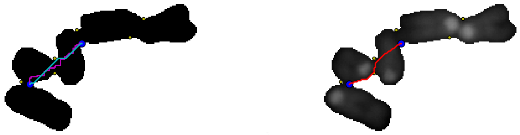
    It should be possible to do better by using a geodesic distance between the points, that is using a path inside the cluster of chromosomes. In the following example:

    On the left, two paths (depending on the chosen pixel neighborhood) between the two blue points were overlaid on a binary image (background is set to 255 and the foreground to 0). The path were determined as follow using skimage 0.8dev:
    graph.route_through_array(negbin ,p1,p2,fully_connected=False)
     or
     graph.route_through_array(negbin ,p1,p2,fully_connected=True)

    • negbin: the negative binary image
    • p1, p2: the two points figured in blue.

    On the right the background (0) was set to 255 (white), the path (red) between the two points was determined by minimizing the "greyscale cost", that is through the valleys between the two points is the image is viewed as a greyscaled landscape.

    All the paths can be determined (left), and then the paths can be sorted according to their cost (right). The four paths with the smallest cost are figured in red (left).


    Download code.

    or see bellow:


    Wednesday, October 24, 2012

    Contour : looking for negatively curved domains

    A contour was previously explored with the convexity defects  algorithm implemented in opencv. Some highly curved domains  failed to be detected because of the contour shape.
    Curved domains missed by convexity defects detection

    Using polygonal approximation imlemented in skimage 0.8 dev, positively curved domains as well as negatively curved domains on a contour can be sorted:
    Contour of a chromosomes cluster (blue), polygonal approximation (yellow). Red points: positive curvature. Yellow points: negative curvature.

    From a segmented particle, a polygonal approximation of the contour is extracted.
    Points of the polygon are used to compute an angle between two consecutive vectors (Here using the complex affix of vectors):

    Positive angles correspond to convex domains and negative angles to concave domains.


    The code has to be modified to filter angles according to a given range. 

    The code can be modified as follow to filter angles corresponding to curved domains:

    • positive = table[(135>table[:,2]) & (table[:,2]>45)]
    • negative = table[(-45>table[:,2]) & (table[:,2]>-135)]
    Curved domains on polygonal approximation of a chromosomes cluster contour.

    Download code


    Thursday, July 19, 2012

    Playing around with opencv convexity defects

    Modifying a little the code of the previous post, removes the points too close to the convex hull:
    Edit the end of the script as follow:

        cv2.line(img,start,end,[255,0,0],1)
        if d>1000:
            cv2.circle(img,far,3,[0,0,255],2)

    Thursday, November 17, 2011

    Thursday, October 20, 2011

    Classifying chromosomes with scikit-learn

    A trained dataset was build from 5 metaphases corresponding to 205 classified chromosomes or nuclei falling in one of four categories: single chromosome, overlapping chromosomes, nuclei or dusts(artefact of image segmentation).  
    Two features were chosen to classify the particles:
    • The particle area (normalised by image size)
    • The convex-hull area of the particle ( area/convex hull). The idea is that particles that are clustered chromosomes will have a smaller ratio than single chromosomes.
    The trained dataset is used to recognise 49 particles segmented from a sixth metaphase and then the predictions from the classifier compared to hand classified particles reached...
                                                                 59.18%

    # -*- coding: utf-8 -*-
    """
    Created on Fri Oct  7 13:08:57 2011
    
    @author: Jean-Patrick Pommier
    """
    import KarIO
    import os
    import pylab
    import pandas
    import numpy as np
    from sklearn import svm
    #make a configurator object
    config=KarIO.ClassifConf()
    #build the the name feature file
    ##list all the feature files
    ##répertoire courant : os.listdir(os.getcwd())
    featurespath=os.path.join(os.getcwd(),"Results","features")
    labelpath=os.path.join(os.getcwd(),"Results","labels")
    #print featurespath
    ##open features csv files
    featuresFilesList=os.listdir(featurespath)
    labelsFilesList=os.listdir(labelpath)
    ##
    metalist=[0,1,2,3,4]
    def makeDataShape(meta):
        featfile=config.user+'-'+config.slide+'-'+config.metaphases_list[meta]+'-'+config.counterstain+'.csv'
        labelfile='shapeCateg-'+featfile
        fea=pandas.read_csv(os.path.join(featurespath,featfile),header=None,index_col=None,names=['particle','ratio','area'])
        lab=pandas.read_csv(os.path.join(labelpath,labelfile),header=None,index_col=None,names=['particle','type'])
        del lab['particle']    
        #merge columns:features and label
        data=fea.join(lab)
        data.insert(0,'meta',int(config.metaphases_list[meta]))
        #print data
        return data
    
    bigdata=makeDataShape(0)
    for meta in metalist:
        bigdata=bigdata.append(makeDataShape(meta),ignore_index=True)
    
    single=bigdata[bigdata['type']=='single']
    touching=bigdata[bigdata['type']=='touching']
    nuclei=bigdata[bigdata['type']=='nuclei']
    dusts=bigdata[bigdata['type']=='dusts']
    
    ##ploting with pylab
    #different colors according to the category
    
    fig=pylab.figure()
    ax = fig.add_subplot(111)
    ax.scatter(single['ratio'],single['area'],c='green',marker='o')
    ax.scatter(touching['ratio'],touching['area'],c='red',marker='o')
    ax.scatter(nuclei['ratio'],nuclei['area'],c='blue',marker='o')
    ax.scatter(dusts['ratio'],dusts['area'],c='pink',marker='o')
    
    #train a classifier
    trainedData=bigdata[bigdata['meta']<15]
    untrained=bigdata[bigdata['meta']>=15]
    print 'trained data'
    print trainedData[:5]
    #extract two columns from trainedData
    #convert to numpy array
    features=trainedData.ix[:,['ratio','area']].as_matrix(['ratio','area'])
    test_features=untrained.ix[:,['ratio','area']].as_matrix(['ratio','area'])
    print 'features'
    print features[:5]
    print 'features shape',features.shape
    print 'features type',type(features)
    ##label is a string:single, touching,nuclei,dust
    print 'labels convertion'
    lab1=trainedData['type']
    print 'lab1',type(lab1)
    f=pandas.Factor(lab1)
    print 'factor f',type(f)
    print 'labels',f.labels[:5]
    print 'labels type',type(f.labels)
    print 'labels shape',f.labels.shape
    #
    ##Classify with sklearn
    classifier = svm.SVC()
    model = classifier.fit(features,f.labels)
    predicted=classifier.predict(test_features)
    
    #match predicted /classified
    hiddenlab1=untrained['type']
    hiddf=pandas.Factor(hiddenlab1)
    match=(predicted==hiddf.labels)
    print"prediction"
    print predicted[:5]
    print 'true classification'
    print hiddf.labels[:5]
    print 'match'
    print match[:5]
    ##Count sucess
    success=np.sum(match[:]==True)
    rate=100.0*success/(1.0*len(match))
    print 'rate of good classification',success,'out of',len(match),'particles'
    print rate,'% success'
    

    Thursday, May 19, 2011

    MFISH image to RGB with image5D

    Wade Schwartzkopf published a MFISH dataset  in 2000. Image5D (a plugin for imagej) can display five different fluorochromes simultaneously:
    Left:raw png images. Top right: RGB image done with Image5D. Bottom right: "karyotype" image with false colors. 

    Far red
    Red
    Spectrum gold
    Spectrum green
    Spectrum aqua
    Dapi
    After chromosome classification, a karyotype image can be produced. This is a grayscaled image associated to a  LUT, to be displayed with false colors:
    Image5D can export a rgb image from the five channels image:
    RGB image generated after background substraction of the five raw images

    Monday, February 7, 2011

    Metaphasic chromosomes segmentation under python

    The following python script implements three ways to segment metaphasic chromosomes through functions relying on scipy.ndimage and pymorph/mahotas. Starting from initial image:

     
    Human DAPI stained metaphasic chromosomes recorded with KAF1600 Peltier cooled CCD camera.
    • The first idea consists in performing a hipass filtering followed by a simple thresholding step and finally cleaning the binary image with a morphological opening. This is achieved with the function def HighPassBinary(image):
    Labelled image displayed with pylab. Hipass filtering results in fragmented nuclei
    •  The second idea, implemented in def metaphaseSeg(image):, tries to preserve both nuclei and chromosomes shape using a region growing algorithm (watershed + markers). The markers are obtained from a regional maxima on a blured DAPI image. However, according to the size of the gaussian kernel the segmented image can be over or under segmented with undetected chromosomes as shown in the following animation:
    gif animation of a region based segmentation with increasing gaussian kernel size (3, 5, 7, 9,11, 13, 19). A small kernel (3) yields an oversegmented image.

    • A third idea tries to combine both methods using the result of the first method as markers to initiate a region growing, implemented in def HighPassMetaphaseSeg(image):
    Artifacts close to the nuclei yield background artifacts near the nuclei.
    The result of this third method wouldn't be too bad if additionnal image cleaning was performed on the first image.
     The python script runs under ubuntu linux , I didn't take care of path to access to the image file to make it portable for windows or MacOS. To use one of the function comment/uncomment the code.

    from scipy import ndimage as ND
    import readmagick
    import mahotas
    import pymorph
    import pylab
    def HighPassBinary(image):
        '''depuis une image DAPI,  genere une image passe haut avec fond a zero'''
        '''necessite scipy.ndimage'''
        blur=ND.filters.gaussian_filter(image, 9)
        sharp=image-1.0*blur
        '''float 64bits'''
        print sharp.dtype, sharp.shape
        smax=sharp.max()
        '''threshold above negative values'''
        imBin=(sharp>0)
        imBin2=ND.binary_fill_holes(imBin)
        imBin3=ND.binary_opening(imBin2, iterations=4)
        labeled,nr_obj=ND.label(imBin3)
        print nr_obj
        return labeled
    
    def metaphaseSeg(image):
        blur=ND.filters.gaussian_filter(image, 15)
        remax=pymorph.regmax(blur)
        binRemax=(remax>0)
        seeds,nr_obj=ND.label(binRemax)
        print nr_obj
        grad=pymorph.gradm(image)
        label=mahotas.cwatershed(grad, seeds, Bc=None, return_lines=False)
        return label
    def HighPassMetaphaseSeg(image):
        '''depuis une image DAPI,  genere une image passe haut avec fond a zero'''
        '''necessite scipy.ndimage'''
        blur=ND.filters.gaussian_filter(image, 9)
        sharp=image-1.0*blur
        '''float 64bits'''
        print sharp.dtype, sharp.shape
        smax=sharp.max()
        '''threshold negative values'''
        imBin=(sharp>0)
        imBin2=ND.binary_fill_holes(imBin)
        imBin3=ND.binary_opening(imBin2, iterations=4)
        seeds,nr_obj=ND.label(imBin3)
        print nr_obj
        grad=pymorph.gradm(ND.filters.gaussian_filter(image, 1))
        labeled=mahotas.cwatershed(grad, seeds, Bc=None, return_lines=False)
        return labeled
       
    if __name__ == "__main__":
        dapi=readmagick.readimg("/home/jeanpat/Applications/Images_test/png/essai09/humain.png")
        '''dapiLabeled=metaphaseSeg(dapi)'''
        dapiLabeled1=HighPassBinary(dapi)
        '''dapiLabeled2=HighPassMetaphaseSeg(dapi)'''
        pylab.imshow(dapiLabeled1)
        pylab.show()
        '''pylab.imshow(dapiLabeled1)
        pylab.show()
        pylab.imshow(dapiLabeled2)
        pylab.show()'''
        '''readmagick.writeimg(dapiBin,"/home/jeanpat/Applications/Images_test/png/essai09/humainBin.png")'''


    Thursday, January 20, 2011

    Labelling chromosome-like shapes using watershed: effect of the chromosome shape

    [edit feb 2013]
    In previous post, the  chromatids of metaphasic chromosomes were labelled by hand with a painting tool in ImageJ following a watershed segmentation step:
    Initial chromatids segmentation in ImageJ after high pass  filtering, thresholding, watershed and image labelling.
    Final chromatids (blue or green) segmentation after painting by hand, centromeric region was added and paint in red.

     With a simplistic rigid model of chromosome and well chosen seeds, a watershed can label the chromatids:

    Chromosomes present variable shapes, metacentric chromosomes are X shaped, acrocentric chromosomes are Y-shaped. The  shape of the same chromosome varies also from one metaphase spread to another, it can be randomly bended,condensed. Image processing introduces also variability according to the parameters used (threshold, filtering ...). Is it possible to segment chromatids such conditions ? Let submit a contour image of chromosome-like shapes to wateshed algorithm implemented in mahotas:

    model shapes of chromosomes of variable size, bending. (Gimp)
    seeds: the darkest seeds will label the back ground, they are outside the chromosomes. The pairs of lighter seeds are supposed to label the chromatids. (The Gimp)
    In a python console:

        PyShell 0.9.8 - The Flakiest Python Shell
        Python 2.6.6 (r266:84292, Sep 15 2010, 15:52:39)
        [GCC 4.4.5] on linux2
        Type "help", "copyright", "credits" or "license" for more information.
        Startup script executed: /home/claire/.pyshell/startup
       >>> g=readmagick.readimg("/home/claire/Applications/ImagesTest/essai02/grad.tif")
       >>> s=readmagick.readimg("/home/claire/Applications/ImagesTest/essai02/seeds.tif")
       >>> label=mahotas.cwatershed(g, s, Bc=None, return_lines=False)
       >>> readmagick.writeimg(label,"/home/claire/Applications/ImagesTest/essai02/label.tif")

    The background is labelled with one seeds outside the chromosomes and with seeds (same grey level) inside the chromosome holes. The chromatids are labelled with one pair of seeds inside the chromosomes:
    Pair of seeds for watershed with two different grey levels


    They are chosen grossly to fall apart the chromosomal axe:

    Labelling with one pair of seeds per chromosome
    If several pair of seeds are chosen by hand, a better chromatid segmentation can be found:
    Pair of seeds overlaid to the particles contour
    Chromatids like segmentation
    The result depends on how the seeds were chosen. Four independent factors seems to be considered:

    • Seeds number:  one pair yields poor results as observed previously.
    • Seeds orientation : the seeds axis, must be locally orthogonal to the axis of the chromosome.
    • For a given pair of seeds, the distance between the two discs.
    • Relative orientation of the pair of seeds: The pair of seeds must have the same orientation.
    When the seeds don't have the same relative orientation, watershed yields an harlequin  pattern :
    opposite pair of seed yield harlequin pattern

    Up to now, image labelling was performed with seeds chosen manually and drawn by hand with the gimp or ImageJ. The seeds localization have to be found automatically and mathematical morphology may provide solutions. The chromosomal axis is close to the particle skeleton. Can the particle skeleton be used to automatically find seeds useful for chromatid labelling with watershed? Using ImageJ interactively, chromosome-like particles skeleton was found:
    chromosome-like particles
    particles skeletons
    From the skeleton, the branching points and end-points are searched using a binary hit-or-miss operator in ImageJ (see here for code). Different hit-or-miss structuring elements suceed in detecting branching points. If end-points and branching points are overlaid on the binary particules, chromosomal areas close to those chosen by hand, are finally found:
    Skeleton branching points (color), skeleton end points (black)
    At first sight end-points would provide better candidate seeds for watershed.