Prune iteratively the leaves of a toy graph with graph-tool

A measure of the similarity of two weighted multigraphs?

To compare shapes, typically obtained after image segmentation, it has been shown that their skeleton could be used. A search with the keywords : skeleton+pruning+image+recognition yields a lot of results.

Assuming that the size of the branches of the skeleton, linking the end-points and the branched points together, can be represented by the weights of the edges in a graph, a weighted graph can represents naturally the skeleton of a shape.

From the skeleton of the B character (left) to its associated (networkx) graph (right).

Previously, pruning of skeletons was performed by removing pixels, one after an other, from the end-points by morphological hit-or-miss. A response curve of a skeleton to pruning, can be defined by counting the end-points of the skeleton as pruning is iterated. It was observed that the responses from similar shapes were similar. So, such response curves may be used to compute some similarity measures, or distances, between shapes.

The time necessary to prune a skeleton depends on its number of pixels. So it may be worth  prior pruning to convert a skeleton into a graph. Thus pruning a graph could be independent from the weight of its edges.

The response of a a weighted multi-graph to iterative pruning was performed with graph-tool (and additionnal python librairies : mahotas, numpy, scipy, matplotlib). This response yields a curve: a "Response to Pruning Curve" or RPC. Then a distance was defined between two RPCs, to compute a similarity index between two graphs.

The graph tool version used is:

2.11 (commit b6b2152c, Mon Oct 26 10:31:30 2015 +0100)

This post summarises the ideas developed in a jupyter notebook.

Algorithm for pruning a graph from its leaves :

1. Make a weighted un-directional multi-graph
2. (Visualize it)
3. Start pruning:
1. Count the vertices on degree 1
2. Read the weight of the edges bound to vertices of degree1 (V1)
3. Get the edge(s) of minimal weight
4. Remove this/these edge(s)
5. Decrease the weight of the other edges bound to vertices v1 by this minimal weight
4.  Do it until no more vertices of degree 1 remains
5. Cumulate the weight of removed edges
6. The response to pruning of a graph, associates the number of degree1 vertices to the cumulative weight of the removed edges.

Make a toy-graph to play with:

By default in graph-tool, the graphs are multi-graphs and that's what we need. The edges of the graph must be weighted, this property has to be created. The weight of an edge corresponds to the size of a branch in a skeleton (the number of pixels). The following python code, shows the creation of a graph with an edge property called 'weight': 

 

The graph can be displayed such that the thickness of its edges maps to the weight of edges:

Start to prune the graph:

Two different versions of the pruning function were written. The second called prune_once_faster() depends on the GraphView() method of the graph-tool library to filter vertices of degree 1, hoping to make a faster function:

The pruning function is destructive, applying it iteratively on the same graph yields, if you write in a jupyter cell:

G0 = make_toy_graph()
g0 = G0.copy()
prune_graph_once(g0)
g1 = g0.copy()
prune_graph_once(g0)
g2 = g0.copy()
prune_graph_once(g0)
g3 = g0.copy()

print G0, number_of_degree1_vertices(G0)
print g1, number_of_degree1_vertices(g1)
print g2, number_of_degree1_vertices(g2)
print g3, number_of_degree1_vertices(g3)

 You will have as output:

<Graph object, undirected, with 4 vertices and 4 edges at 0x9c65c1ac> 2
<Graph object, undirected, with 4 vertices and 3 edges at 0x9c65cc2c> 1
<Graph object, undirected, with 4 vertices and 2 edges at 0x9c654dec> 1
<Graph object, undirected, with 4 vertices and 1 edge at 0x9c65424c> 0

 Indicating that the number of edges decreases as the number of vertices of degree 1, each time the graph is pruned.

Pruning iteratively a graph: 

Let's count the number of vertices of degree 1 as the graph is pruned. The toy graph used here to check its response, has two vertices of degree 3 and two vertices of degree 1 (vertices 2 an 3). The initial values of the weight of the edges bound to vertices 2 and 3, are :

15, 20

The smallest weight is 15 So after one pruning, the weights becomes:

15-15 = 0, 20-15 = 5

The edge 1-2 of weight 0 is removed (vertex 2 is now of degree 0). 

The edge 1-3 has the smallest weight (5). 

So after a second round of pruning, the edge 1-3 is removed.

The vertex 1 was of degree 2, now it is of 1. The weight of the edge 0-1 is 8.

A third pruning removes the last edge 0-1 of weight equal to 8.

The degree of vertex 0 is 2 (there's a loop), so the edge 0-0 can't be pruned. The different weights are cumulated as follow:

0, 15, 15+5, 20+8

Applied to a skeleton made of pixels, this would mean that:

• 15 prunings of 1 pixel would remove one branche of size 15.

• 20 prunings would remove the two branches of size 15 and 20.

• 28 prunings would remove the three branches of sizes 15, 20 and 8 (initially between two vertices of degree 3).

The weights are stored in a vector X .

The corresponding counts of degree 1 vertices are stored in a vector Y.

Both X,Y are returned by the function response_to_iterative_pruning()

Make a feature vector from the pruning curve?

A response curve was plotted as a step curve:

The upper curve is the response when the weight of edges are used. In the lower one, the weights were normalised by the total weights of the graph (% total length or total weight), hopping to produce a scale invariant response. For the following, only the raw response will be used.

Distance between two graphs:

First, we need new toy graphs to compare them. The second new graph differe from the first only by its weight:

The third one has no loop:

 A fourth has a loop elsewhere:

The response of the three first graphs are:

Overlayed responses of first and third graph (right)

We could try to compute the area between two step curves. For two identical curves the area would be null, as the curves differe the area may increase. Fine!

However, the curves are just defined from discrete data, it may not be so easy to define for such kind of integration.

Let's forget the curves and just look at the points from the scatter plot. When looking at two pruning curves obtained from toy-graphs 2 and 3, we could just compute the distances matrix between the points from the two curves. The more the curves are different, the more the distances should increase ... why not, give it a try:

scipy provides just what we need!

The response curve is given as (X, Y) with

• X : The pruning values 

• Y : the corresponding number of leaf in the graph (vertices of degree 1)

First, let's compute the distances between the points of the same curve:

T=make_toy_graph()
X, Y = response_to_iterative_pruning(T.copy())
pruning_curve = zip(X,Y)
D = cdist( pruning_curve, pruning_curve)
print D

Thanks to scipy, we get a 4x4 (since the graph has four vertices) matrix of distances D :

[[  0.          15.03329638  20.02498439  28.0713377 ]
 [ 15.03329638   0.           5.          13.03840481]
 [ 20.02498439   5.           0.           8.06225775]
 [ 28.0713377   13.03840481   8.06225775   0.        ]]

Which can be displayed as an image (the matrix is symetric, only upper element are displayed):

For each of the three first graphs T,T1,T2 , one can define 32−32+3=6   matrices of distances.

Those matrices are elements of another matrix (a matrix of matrices). The elements of the diagonal are squared matrices corresponding to "intra-distances" (distances between the points of the same response curve).

The elements outside the diagonal correspond to "inter-distances" matrices (distances computed from points belonging to two different response curves), the "inter-distance matrices", here, can be  rectangular if the corresponding pairs of graphs do not have the same number of vertices (and square if the two graphs have the same number of vertices):

 For each matrix, the total distance can be computed as the sum of their elements. This yields:

[[ 178.  187.  256.]
 [   0.  105.  135.]
 [   0.    0.  140.]]

At first sight, this is not good, elements outside the diagonal (total distance between two response curves, that is the distance between two graphs)  should be greater than those of the diagonal.

Defining a normalized distance between two graphs

We try to heal this situation by normalising the inter-distances . The total inter-distances is normalized by the sum of total intra-distances. The total inter distances is multiplied by two in order to have a normalised distance:
 nD .  

nD(responsecurvei,responsecurvei)=1

When computed against the pair of same response curve, the normalized distance equals 1 as wished.

Finally nD  is computed as follow:

nD(ri,rj)=12distance(ri,rj)ri+rj=ri+rj2distance(ri,rj)

such that:

nD(ri,rj)<=1

Let's see the matrix of normalised distance on the three first graphs:

[[ 1.          0.75751403  0.62186779]
 [ 0.          1.          0.90636131]
 [ 0.          0.          1.        ]]

As an image:

This seems better. With that distance, the similarity of a graph on itself is 1 and two different graphs have a similarity bellow 1. It remains to see if that distance can discriminate between graphs of interest possibly after supervised classification.

Graph again

Update 06 /11 /2014

The ipython notebook from the previous post was rewritten . A python  function building a graph from a skeleton was modified to generate a multigraph (networkx). This function (available in an ipython notebook) is used as follow:

    Graph= nx.MultiGraph()
    C8_Skeleton_To_Graph_01(Graph, skeleton)

With:

• Graph : a networkx multigraph object.
• skeleton : the binary image of skeleton obtained by morphological thining with mahotas.

In the following example (from the previous ipython notebook), the skeleton of the letter 'a' was converted into a networkx multigraph: 

image_test= makeLetterImage('a', 75)
skeleton_test = mh.thin(image_test)
_,_,Bp_test,Ep= SkeletonDecomposition(skeleton_test)
Ep_Ep = skeleton_test*np.logical_not(Ep)
Ep_Ep,_ = mh.label(Ep,Ep)
l_Ep, _ = mh.label(Ep)


Graph_test = nx.MultiGraph()
C8_Skeleton_To_Graph_01(Graph_test, skeleton_test)
print Graph_test.edges(data=True)

figsize(16,8)
subplot(131)
imshow(skeleton_test+l_Ep+3*Bp_test,interpolation='nearest')
subplot(132, xticks=[],yticks=[])
nx.write_dot(Graph_test,'multi.dot')
!neato -T png multi.dot > multi.png
imshow(mh.imread('multi.png'), interpolation='nearest')
subplot(133)
nx.draw(Graph_test)

The skeleton has two edges, linking the same branched points (yellow and red pixels). The graph was exported to build an image of the multigraph (middle), networkx doesn't seem to be capable to dispolay correctly such multigraph (right)

When applied to a lowercase alphabet:

The function produced the corresponding graphs (the letter 'o' excepted):

However,it is possible to find case where the function failed to buil a graph as:

   imTest = makeLetterImage('b', 70)
   skelTest = mh.thin(imTest)
   Ep_Bp, Bp_Bp, Bp, Ep = SkeletonDecomposition(skelTest)

where:

• skeltest: the image skeleton obtained by thining with mahotas.
• Bp : image of branched-point(s)
• Ep: image of end-point(s)
• Bp_Bp :edge(s) between branched-points
• Ep_Bp:edge(s) between end-point(s) and branched-point(s)

If the skeleton of the letter 'b' is decomposed as follow:

The function fails to produce a graph due to the presence of a closed edge (right) which should be processed as a self loop for the corresponding branched-point (middle image).

An other graph library: Graph-tool

The graphic representation of a multigraph produced by graphtool is so nice that it may worth to learn the graphtool syntax to make a graph:

Construct a graph from the skeleton image of a binary form

Previously an attempt was made to write a code capable of building a graph from the skeleton of an image and it was not a complete success since some preprocessing (pruning) had to be done to build a graph. Here an other python code was written and at very first sight, it seems to produce a graph without complaining....sometimes (see at the end).

The code was run in a ipython notebook running on sagemath cloud. It relies on several libraries : mahotas and networkx, numpy is provided by default. Scikit image was also tested. Pillow was used to generate images of some letter as model.

The idea is the following:

• make the skeleton of a binary image.
• get its branched-points and add them in a graph.
• get its end-points, add them to the graph.
• get the edges of the skeleton and decompose them into:
• edges between end-points and branched-points.
• edges between branched points.
• add edges to the graph between end-points and branched-points.
• add edges to the graph between branched-points.

Images models

Since the code is run on sagemath cloud, Pillow has to be installed. From a terminal :

pip install Pillow

 The verdana true type font was obtained from fontsupply and the file verdana.ttf had to be at the same location than the ipython notebook ( verdana.ttf was uploaded on SMC project at the same location than the ipython notebook).

The code used to generate images and draw them is:

and we get:

What kind of skeleton?

Both mahotas an scikit-image implement morphological operators to generate the skeleton of a binary shape. Scikit-image seems to use a neighbourhood  on 4 pixels (C4) and mahotas on on neighbourhood of 8 pixels (C8). This is why mahotas was retained to produce skeletons:

• medial axis  of the letter A computed with scikit image (left), branched points and end-points are extracted using hit-or-miss operator implemented in mahotas (middle). The branched-points can be removed from the medial axis and the resulting image can be labelled (left), pixels connected only vertically or horizontally share the same label.

Skeleton from the letter A (left)

•  If a skeleton is generated by morphological thining with mahotas, we get the left image. The fourth image is the skeleton deprived of its branched points. Scikit-image provide a thining operator with a C4 neighborhood (right image):

 

C8 skeleton by thining (left). C4 skeleton by thining (right).

What's happen if a C8 skeleton is labeled? Here, both mahotas and scikit-image provide the same result:

edges (mahotas:left; scikit-image:right)

The labelled regions fit here what can be seen as an edges.

Prior to start to build a graph, several additionnal images are needed:

Edges decomposition:

Let's decompose the image of edges by considering edges connecting end-points to branched-points and edges connecting only branched points:

Starting to build the graph by the branched-points:

 The branched-points are added first. The branched point of label 1 in the image, is the first vertex in the graph, and so on:

The end points are the added to the graph, there is a shift between the end-points label in the image and their index in the graph. The first end-point in the image will be the fith vertex in the graph:

The vertex of the graph (G) have attributes derived from the images they come from: their position 'pos' define by (row,col), their label in the image of origin. Typing in a ipython cell:

          print G.nodes(data=True)
          print nx.get_node_attributes(G,'label')

yields:

[(1, {'pos': (3, 9), 'label': 1}), (2, {'pos': (3, 12), 'label': 2}), (3, {'pos': (17, 5), 'label': 3}), (4, {'pos': (17, 17), 'label': 4}), (5, {'pos': (1, 9), 'label': 1}), (6, {'pos': (1, 13), 'label': 2}), (7, {'pos': (25, 3), 'label': 6}), (8, {'pos': (25, 21), 'label': 8})]
{1: 1, 2: 2, 3: 3, 4: 4, 5: 1, 6: 2, 7: 6, 8: 8}

Linking end-points to branched points:

 The idea here is to get the neighbourhood of each branched-point in the "edges ep-ep" image and to add an edge in the graph between the corresponding branch-point and end-point(s). This yield:

Linking branched-points

•  A dictionnary where the keys are the labels of the branched-points and the values are the label of the "edges bp-bp" in the neighbourhood of the branched point is build. Thus there's one key (bp label) for several values (edges labels).
• But an edge can be seen as one key (the edge label) for two values (the two labels of the two branched-points). So the dictionnary has to be inverted in that very particular way. Fortunately, that problem was solved on stackoverflow.

 Finaly, we have:

 the whole steps are gathered in a function:

Processing other  letters gives for example:

The ipython notebook is here:

View the notebook on ipython.org

Sometimes building the graph fails:

On a larger set of images:

• For the image corresponding to the letter K, the graph construction fails due to the presence of branched regions made of several pixels instead of one.
• There's also a problem with the letter D, its graph has no loop.
• Since there's no branched point in the skeleton of the letter C, its graph is not build.

 The ipython notebook has been reordered and is available on ipython.org

Which structuring elements to detect branched points?

In a 2D skeleton obtained after thinning of a binary image, pixels having 3 or 4 (or more...) neighbors are branched-points. Hit-or-miss operator can be used to detect branched points (or junction points). Structuring elements, SE, can be 3x3 arrays representing the pixels configuration to be detected. Here different 3x3 structuring elements were explored on some simple test images with the hit-or-miss operator implemented in mahotas 1.0 .

• There are two SE to detect pixels with 4 neighbors, called here X0 and X1.
• There are two set of SE detecting pixels with at least 3 pixels, a Y-like configuration and a T-like configuration. Each of these configurations can be rotated by 45°, making 16 different SE.

18 SE were found , since don't care pixels were used a branched points can be detected by different SE, a pixel detected by X0 should be detected by T4 too. The 18 SE can be displayed as 3x3 image:

Black:background pixel (0), Blue: foreground pixel (1), Red:Don't care pixel (0 or 1)

Applied on a small skeleton-like test image (left), two branched-points  (junction) and four end-points are detected:

On a larger image, from the SIID images database:

Hit-or-miss transformation applied on the skeleton (up right), yields end-points (lower right). Since the same branched-points can be detected by different structuring elements, branched points appear of a variable color according to the detection occurence. Moreoever, branched-points can be connected yielding a branched domain of pixels.

ipython notebook

HMT-SE.ipynb

From binary image skeleton to networkx graph.

To recognize objects in an image methods involving graphs have been developped as the shock graph method. These graphs are derived from image skeleton and then handled, compared. However, it seems taken for granted that a graph is available for work.

Here is proposed a python code generating a networkx graph object from the skeleton of a binary image.

The image of the B letter was chosen as model. The image is generated with PIL:

Skeleton decomposition:

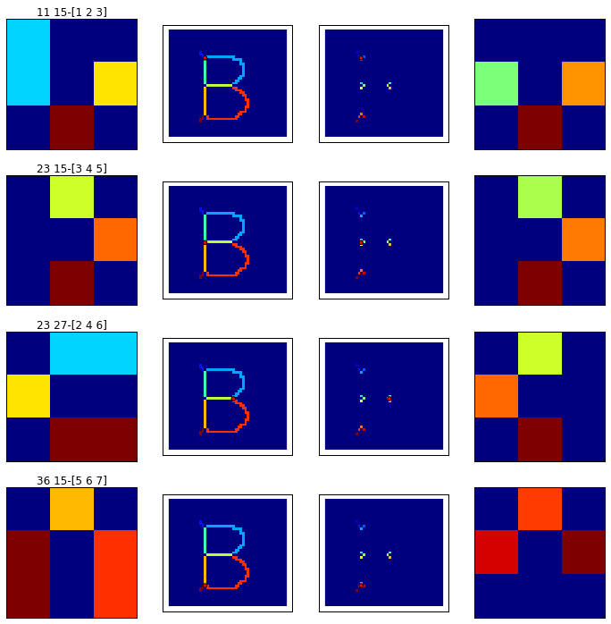
The shape skeleton is computed by morphological thining, branched points are extracted from the skeleton with a hit-or-miss operator and labelled:

Finding the neighborhood of the branched points:

• The end points are extracted and labelled from the initial skeleton (top left image) .

• The edges are obtained by difference between the skeleton of the shape and the branched points of the skeleton. Seven edges were found and labelled from 1 to 7 (middle left image).

• The edges are pruned by one pixel, the labels values are 1,2,3,4,5,6,7 (middle right image).

• The edges end points are then extracted and labelled individually (1,2,3,...,14) (bottom left image).

• The end points are also labelled according to their edge of origin ( 1,2,3,4,5,6,7), (bottom right image).

For each branched point, its neighborhood is isolated to get the labels of the adjacent end points (right images):

Building the graph:

The graph is build by adding branched points first (vertex 1, 2, 3, 4), it assumes that at least one branched point exists, then  end points adjacent to the branched points are added (vertex 8,9,10 and 11,12,13 and 14,15,16): 

The remaining lonely end points are added to the graph (vertex 17, 18):

The end points are linked using the pruned edges, the edges are weighted according to their pixel size:

Graph of the letter B, without initial skeleton pruning. The edges length here do not match to their weight

A bug somewhere (update fri 06, 2013):

For some shapes, as 'Y':

The algorithm fails at the end points linking step. A way to cure the situation is to prune the initial skeleton of 'Y' once:

 

In the case of the letter 'A', the skeleton must be pruned three times for the algorithm to succeed:

Bug origin:

With the letter 'Y', with initial skeleton pruning, the algorithm yields the following graph:

Branched points are figured in red circles on the image of labelled edges and end points are figured by a white star.

In the case of the letter 'A', the algorithm yields :

The bug seems to come from too short edges as after three pruning steps removing the small barbs on the top of the letter, the algorithm succeeds in producing a graph

Download ipython notebook

 ipython notebook available at ipython.org
or from gist: