Looking for a geodesic distance to resolve touching chromosomes

In the previous post, from a cluster of touching mouse chromosomes:

DAPI stained mouse chromosomes

points belonging to negatively curved domains of a contour can be isolated :

To separate the chromosomes, it is tempting to cut between the closest pairs of points.

Python provides itertools.combinations(); the closest pairs of points are in the set of the combinations of every pairs of points:

Each line shows the euclidian distance between two points, the four shortest lines correspond more or less to the contact domains between the chromosomes, cuting along them provides a way to separate the chromosomes.

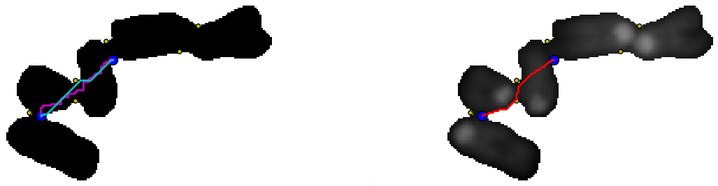
It should be possible to do better by using a geodesic distance between the points, that is using a path inside the cluster of chromosomes. In the following example: two paths (depending on the chosen pixel neighborhood) between the two blue points were overlaid on a binary image (background is set to 255 and the foreground to 0).

the cluster contourthe cluster contour

 The path were determined as follow using skimage 0.8dev:

graph.route_through_array(negbin ,p1,p2,fully_connected=False)

 or

 graph.route_through_array(negbin ,p1,p2,fully_connected=True)

 with negbin, the negative binary image and p1, p2 the two points figured in blue.

If the background (0) is set to 255 (white) in the grey scale image:

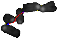
 the path (red) between the two points can be determined by minimizing the "greyscale cost", that is through the valleys between the two points is the image is viewed as a landscape.

All the paths can be determined (blue):Those paths in blue were obtained from the previous binary image:

The paths were sorted according to their cost :

 The four paths with the smallest cost are figured in red, they are "inside" the cluster. Some paths are partially "outside" the cluster and thus are not geodesic routes inside the cluster.
Now if paths are calculated from a 8 bits greyscale image where the background was set to 255 (a naïve idea supposed to prevent a path to go "outside" a cluster):

some routes between two points, go along the contour. The two first routes to with the smallest costs do correspond to touching domains between the chromosomes. However when routes with higher cost are selected:

some correspond to the cluster contour and not to contact domains between the chromosomes, because the cost (sum of pixels grey value) along the contour is probably lower than the cost of a shorter path which have to climb over a contact domain between two chromosomes.

Additional features may distinguish routes belonging to contour from those providing solution to separate chromosomes:

red route on the right resolve touching chromosomes

Minimal cost routes are still better to separate chromosomes than routes obtained with euclidian distance:

The shortest path (on the right) cuts inside the chromosome

Download code

Trying to separate touching mouse chromosomes

In the previous post, from a cluster of touching mouse chromosomes:

points belonging to negatively curved domains of a contour can be isolated :

Yellow points belong to negatively curved domains of the contour.

To separate the chromosomes, it is tempting to cut between the closest pairs of points.

Let's make combination of pairs of points belonging to the contour:

Python provides itertools.combinations(); the closest pairs of points are in the set of the combinations of every pairs of points:

Path between two points belonging to the countour:

Each line shows the euclidian distance between two points, the four shortest lines correspond more or less to the contact domains between the chromosomes, cuting along them provides a way to separate the chromosomes.

It should be possible to do better by using a geodesic distance between the points, that is using a path inside the cluster of chromosomes. In the following example:

On the left, two paths (depending on the chosen pixel neighborhood) between the two blue points were overlaid on a binary image (background is set to 255 and the foreground to 0). The path were determined as follow using skimage 0.8dev:

graph.route_through_array(negbin ,p1,p2,fully_connected=False)

 or

 graph.route_through_array(negbin ,p1,p2,fully_connected=True)

• negbin: the negative binary image
• p1, p2: the two points figured in blue.

On the right the background (0) was set to 255 (white), the path (red) between the two points was determined by minimizing the "greyscale cost", that is through the valleys between the two points is the image is viewed as a greyscaled landscape.

All the paths can be determined (left), and then the paths can be sorted according to their cost (right). The four paths with the smallest cost are figured in red (left).

Download code.

or see bellow:

Contour : looking for negatively curved domains

A contour was previously explored with the convexity defects  algorithm implemented in opencv. Some highly curved domains  failed to be detected because of the contour shape.

Curved domains missed by convexity defects detection

Using polygonal approximation imlemented in skimage 0.8 dev, positively curved domains as well as negatively curved domains on a contour can be sorted:

Contour of a chromosomes cluster (blue), polygonal approximation (yellow). Red points: positive curvature. Yellow points: negative curvature.

From a segmented particle, a polygonal approximation of the contour is extracted.

Points of the polygon are used to compute an angle between two consecutive vectors (Here using the complex affix of vectors):

Positive angles correspond to convex domains and negative angles to concave domains.

The code has to be modified to filter angles according to a given range. 

The code can be modified as follow to filter angles corresponding to curved domains:

• positive = table[(135>table[:,2]) & (table[:,2]>45)]

• negative = table[(-45>table[:,2]) & (table[:,2]>-135)]

Curved domains on polygonal approximation of a chromosomes cluster contour.

Download code

Playing around with opencv convexity defects

Modifying a little the code of the previous post, removes the points too close to the convex hull:

Edit the end of the script as follow:

    cv2.line(img,start,end,[255,0,0],1)
    if d>1000:
        cv2.circle(img,far,3,[0,0,255],2)

Convexity defects in a cluster of mouse chromosomes

Just a little trial to explore cv2.convexityDefects() on a cluster of mouse chromosomes:

The cluster consists in five touching mouse chromosomes. The aim is to use cv2 to display the contour of the particle, its convex hull, and to see what it is possible to do with convexityDefects function implemented in OpenCv 2.4.2 which provides now the big advantage of handling numpy array. The python script used is largely inspired from abid rahman's blog:

# -*- coding: utf-8 -*-
"""
Created on Wed Jul  4 14:43:42 2012

@author: jean-pat
"""

import cv2
import numpy as np
import os
import pylab as plb
print cv2.__version__

user=os.path.expanduser("~")
workdir=os.path.join(user,"QFISH","JPPAnimal","JPP52","11","DAPI","particles")

file="part25.png"
complete_path=os.path.join(workdir,file)

img = cv2.imread(complete_path)
gray = cv2.cvtColor(img,cv2.COLOR_BGR2GRAY)
ret,gray = cv2.threshold(gray,1,255,0)
print ret
gray2 = gray.copy()
mask = np.zeros(gray.shape,np.uint8)

contours, hier = cv2.findContours(gray,cv2.RETR_LIST,cv2.CHAIN_APPROX_SIMPLE)
print hier
cv2.drawContours(img,contours,0,(0,255,0),1)
cnt = contours[0]
hull = cv2.convexHull(cnt,returnPoints = False)
#print hull
approx = cv2.approxPolyDP(cnt,0.05*cv2.arcLength(cnt,True),True)
print 'approx',approx

print 'contours',type(cnt), cnt.dtype, len(contours)
defects = cv2.convexityDefects(cnt,hull)
print defects
for i in range(defects.shape[0]):
    s,e,f,d = defects[i,0]
    start = tuple(cnt[s][0])
    end = tuple(cnt[e][0])
    far = tuple(cnt[f][0])
    cv2.line(img,start,end,[255,0,0],1)
    cv2.circle(img,far,5,[0,0,255],1)

plb.imshow(img)
plb.show()

    

The result is :

Strangely, some convexity defects (blue circles) of the particle contour (green curve) are very close to the particle convex hull (red curve). Four defects are detected on the contour where the chromosomes touch each other as waited. Those contact regions correspond to "neck" on the contour curve, and only one side of the neck is detected.
At first sight, there is nine false positive points, four well detected points and four non detected points (the other side of the "necks").

From the script, the content of the defect variable is:

[[[  214   216   215   689]]
[[  216   218   217   114]]
[[    0    30    19  2444]]
 [[   30    32    31   234]]
 [[   32    34    33   201]]
 [[   34    38    37   278]]
 [[   38    71    56  5658]]
 [[   72    78    73   114]]
 [[   78    94    87  3133]]
 [[   96    98    97   114]]
 [[   98   106   101   297]]
 [[  106   120   111   364]]
 [[  121   212   179 12452]]]

The convexity defect is a list of vectors of the form:

(start_index, end_index, farthest_pt_index, fixpt_depth)

so it should be possible to filter the points too close to the convex hull.