Construct a graph from the skeleton image of a binary form

Previously an attempt was made to write a code capable of building a graph from the skeleton of an image and it was not a complete success since some preprocessing (pruning) had to be done to build a graph. Here an other python code was written and at very first sight, it seems to produce a graph without complaining....sometimes (see at the end).

The code was run in a ipython notebook running on sagemath cloud. It relies on several libraries : mahotas and networkx, numpy is provided by default. Scikit image was also tested. Pillow was used to generate images of some letter as model.

The idea is the following:

• make the skeleton of a binary image.
• get its branched-points and add them in a graph.
• get its end-points, add them to the graph.
• get the edges of the skeleton and decompose them into:
• edges between end-points and branched-points.
• edges between branched points.
• add edges to the graph between end-points and branched-points.
• add edges to the graph between branched-points.

Images models

Since the code is run on sagemath cloud, Pillow has to be installed. From a terminal :

pip install Pillow

 The verdana true type font was obtained from fontsupply and the file verdana.ttf had to be at the same location than the ipython notebook ( verdana.ttf was uploaded on SMC project at the same location than the ipython notebook).

The code used to generate images and draw them is:

and we get:

What kind of skeleton?

Both mahotas an scikit-image implement morphological operators to generate the skeleton of a binary shape. Scikit-image seems to use a neighbourhood  on 4 pixels (C4) and mahotas on on neighbourhood of 8 pixels (C8). This is why mahotas was retained to produce skeletons:

• medial axis  of the letter A computed with scikit image (left), branched points and end-points are extracted using hit-or-miss operator implemented in mahotas (middle). The branched-points can be removed from the medial axis and the resulting image can be labelled (left), pixels connected only vertically or horizontally share the same label.

Skeleton from the letter A (left)

•  If a skeleton is generated by morphological thining with mahotas, we get the left image. The fourth image is the skeleton deprived of its branched points. Scikit-image provide a thining operator with a C4 neighborhood (right image):

 

C8 skeleton by thining (left). C4 skeleton by thining (right).

What's happen if a C8 skeleton is labeled? Here, both mahotas and scikit-image provide the same result:

edges (mahotas:left; scikit-image:right)

The labelled regions fit here what can be seen as an edges.

Prior to start to build a graph, several additionnal images are needed:

Edges decomposition:

Let's decompose the image of edges by considering edges connecting end-points to branched-points and edges connecting only branched points:

Starting to build the graph by the branched-points:

 The branched-points are added first. The branched point of label 1 in the image, is the first vertex in the graph, and so on:

The end points are the added to the graph, there is a shift between the end-points label in the image and their index in the graph. The first end-point in the image will be the fith vertex in the graph:

The vertex of the graph (G) have attributes derived from the images they come from: their position 'pos' define by (row,col), their label in the image of origin. Typing in a ipython cell:

          print G.nodes(data=True)
          print nx.get_node_attributes(G,'label')

yields:

[(1, {'pos': (3, 9), 'label': 1}), (2, {'pos': (3, 12), 'label': 2}), (3, {'pos': (17, 5), 'label': 3}), (4, {'pos': (17, 17), 'label': 4}), (5, {'pos': (1, 9), 'label': 1}), (6, {'pos': (1, 13), 'label': 2}), (7, {'pos': (25, 3), 'label': 6}), (8, {'pos': (25, 21), 'label': 8})]
{1: 1, 2: 2, 3: 3, 4: 4, 5: 1, 6: 2, 7: 6, 8: 8}

Linking end-points to branched points:

 The idea here is to get the neighbourhood of each branched-point in the "edges ep-ep" image and to add an edge in the graph between the corresponding branch-point and end-point(s). This yield:

Linking branched-points

•  A dictionnary where the keys are the labels of the branched-points and the values are the label of the "edges bp-bp" in the neighbourhood of the branched point is build. Thus there's one key (bp label) for several values (edges labels).
• But an edge can be seen as one key (the edge label) for two values (the two labels of the two branched-points). So the dictionnary has to be inverted in that very particular way. Fortunately, that problem was solved on stackoverflow.

 Finaly, we have:

 the whole steps are gathered in a function:

Processing other  letters gives for example:

The ipython notebook is here:

View the notebook on ipython.org

Sometimes building the graph fails:

On a larger set of images:

• For the image corresponding to the letter K, the graph construction fails due to the presence of branched regions made of several pixels instead of one.
• There's also a problem with the letter D, its graph has no loop.
• Since there's no branched point in the skeleton of the letter C, its graph is not build.

 The ipython notebook has been reordered and is available on ipython.org

From binary image skeleton to networkx graph.

To recognize objects in an image methods involving graphs have been developped as the shock graph method. These graphs are derived from image skeleton and then handled, compared. However, it seems taken for granted that a graph is available for work.

Here is proposed a python code generating a networkx graph object from the skeleton of a binary image.

The image of the B letter was chosen as model. The image is generated with PIL:

Skeleton decomposition:

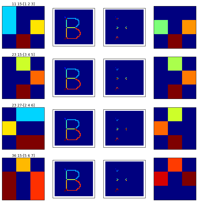
The shape skeleton is computed by morphological thining, branched points are extracted from the skeleton with a hit-or-miss operator and labelled:

Finding the neighborhood of the branched points:

• The end points are extracted and labelled from the initial skeleton (top left image) .

• The edges are obtained by difference between the skeleton of the shape and the branched points of the skeleton. Seven edges were found and labelled from 1 to 7 (middle left image).

• The edges are pruned by one pixel, the labels values are 1,2,3,4,5,6,7 (middle right image).

• The edges end points are then extracted and labelled individually (1,2,3,...,14) (bottom left image).

• The end points are also labelled according to their edge of origin ( 1,2,3,4,5,6,7), (bottom right image).

For each branched point, its neighborhood is isolated to get the labels of the adjacent end points (right images):

Building the graph:

The graph is build by adding branched points first (vertex 1, 2, 3, 4), it assumes that at least one branched point exists, then  end points adjacent to the branched points are added (vertex 8,9,10 and 11,12,13 and 14,15,16): 

The remaining lonely end points are added to the graph (vertex 17, 18):

The end points are linked using the pruned edges, the edges are weighted according to their pixel size:

Graph of the letter B, without initial skeleton pruning. The edges length here do not match to their weight

A bug somewhere (update fri 06, 2013):

For some shapes, as 'Y':

The algorithm fails at the end points linking step. A way to cure the situation is to prune the initial skeleton of 'Y' once:

 

In the case of the letter 'A', the skeleton must be pruned three times for the algorithm to succeed:

Bug origin:

With the letter 'Y', with initial skeleton pruning, the algorithm yields the following graph:

Branched points are figured in red circles on the image of labelled edges and end points are figured by a white star.

In the case of the letter 'A', the algorithm yields :

The bug seems to come from too short edges as after three pruning steps removing the small barbs on the top of the letter, the algorithm succeeds in producing a graph

Download ipython notebook

 ipython notebook available at ipython.org
or from gist:
 

Getting the neighborhood of labelled particles in a graph

In the previous post, a labelled image, typically obtained by labelling connected components of a binary image, was used to compute a dictionary representing the neighborhood relationships between the particles.

A dictionary may be not the best data structure to represent such relationship. A graph structure is better suited and networkx provides a python implementation for that.

Starting from the following label image:

Background Grey level=0, first particle: grey level=1, ...last particle:grey level=5

We get two possible graphs. The first one takes the background (vertex 0) into account so the background is a neighbour of all the particles (there an edge between the vertex 0 and all the other vertex)

In this second graph, the background was removed:

A function  converts the dictionary to a networkx graph:

# -*- coding: utf-8 -*-
"""
Created on Mon Jun 25 10:26:01 2012

@author: Jean-Patrick Pommier
"""

import numpy as np
import networkx as nx
import mahotas as mh
import pylab as plb 

def makelabelarray():
    label = np.array([[0,1,4,4],
                     [1,0,0,2],
                     [3,0,2,2],
                     [0,2,0,5]])
    return label

def convertToGraph(dic, noBack=True):
    G = nx.Graph()
    G.add_nodes_from(dic.keys())
    for particle in dic.keys():
        list_touching_particles = dic[particle]
        # remove background
        if noBack:
            list_touching_particles.discard(0) 
        print 'v(',particle,')=',list_touching_particles
        for tp in list_touching_particles:
            G.add_edge(particle,tp)
    return G
    
def findneighborhoods(label,neighborhood):
    ''' given a labelled image, should return the adjacency list
        of particles, for a given neighborhood:
        
        neighborhood=np.array([0,1,0],[1,1,1],[0,1,0])
        
        The background (0), is kept as a particle neighbor 
        No fancy indexing
    '''
    #make the labels list
    labmax = label.max()
    #print labmax
    neighb_dic = {} # a dictionnary containing particle label as key and neighborhood
    for i in range(1,labmax+1):
        mask = (label ==i)
        #print mask
        dilated = mh.dilate(mask,neighborhood)
        neighbor = np.logical_and(dilated, np.logical_not(mask))
        #print neighbor
   #=======================================================================
        flatlab = np.ndarray.flatten(label)
        flatneighborhood = np.ndarray.flatten(neighbor)        
        flatneighbors = flatlab[flatneighborhood]
        flatneighbors.sort()
        #set is a trick so that each value of the neighborhoods is present only once
        neighb_dic[i] = set(flatneighbors)
        #print np.nonzero(flatneighbors)
    return neighb_dic
        
if __name__ == "__main__":
    a = makelabelarray()
    n = np.array([[1,1,1],[1,1,1],[1,1,1]])
    g = findneighborhoods(a, n)
    G = convertToGraph(g, noBack=True)

    plb.imshow(a,interpolation = 'nearest')
    plb.colorbar(ticks=[0,1,2,3,4])
    plb.show()

    nx.draw(G)
    plb.show()
    
        

Neighbourhood in a labelled image

Image segmentation can yield labelled images, where the different labels correspond to the objects of interest ( chromosomes, a nuclei ). 

It can be necessary to consider particles in the neighbourhood of a given particle. 

The following 4x4 labelled image (a numpy array) is made of four particles:

• first particle : light blue (value or label=1)
• second particle : green (value=2)
• third particle : orange (value=3)
• fourth particle : red (value=4)
• background : dark blue (value = 0)

Considering a 3x3 domain (in fact a structuring element), the neighbour particle of the first particle is the 'orange' particle. The 'orange' particle has two neighbours, the 'light blue' and the 'green' particle .

The following python script takes a label image (from the above example) and returns a dictionary, where  in the  key/value pair, the key corresponds to a chosen particle and the value to a set containing the label value of the neighbouring particles:

{1: set([0, 3]), 2: set([0, 3, 4]), 3: set([0, 1, 2]), 4: set([0, 2])}

The calculated dictionary is closed to an adjacency list.

# -*- coding: utf-8 -*-
"""
Created on Mon Jun 25 10:26:01 2012

@author: Jean-Patrick Pommier
"""

import numpy as np
import mahotas as mh
import pylab as plb 

def makelabelarray():
    label = np.array([[0,1,0,0],
                     [1,0,0,2],
                     [3,0,2,2],
                     [0,2,0,4]])
    return label

def findneighborhoods(label,neighborhood):
    ''' given a labelled image, should return the adjacency list
        of particles, for a given neighborhood:
        
        neighborhood=np.array([1,1,1],[1,1,1],[1,1,1])
        
        The background (0), is kept as a particle neighbor 
        No fancy indexing
    '''
    #make the labels list
    labmax = label.max()
    #print labmax
    neighb_dic = {} # a dictionnary containing particle label as key and neighborhood
    for i in range(1,labmax+1):
        mask = (label ==i)
        #print mask
        dilated = mh.dilate(mask,n)
        neighbor = np.logical_and(dilated, np.logical_not(mask))
        #print neighbor
#==============================================================================
#         #Done without fancy indexing
#==============================================================================
        flatlab = np.ndarray.flatten(label)
        flatneighborhood = np.ndarray.flatten(neighbor)        
        flatneighbors = flatlab[flatneighborhood]
        flatneighbors.sort()
        #set is a trick so that each value of the neighborhoods is present only once
        neighb_dic[i] = set(flatneighbors)
        #print np.nonzero(flatneighbors)
    return neighb_dic
        
if __name__ == "__main__":
    a = makelabelarray()
    n = np.array([[1,1,1],[1,1,1],[1,1,1]])
    print findneighborhoods(a, n)
    plb.imshow(a,interpolation = 'nearest')
    plb.show()