Friday, October 26, 2012

Trying to separate touching mouse chromosomes

In the previous post, from a cluster of touching mouse chromosomes:


points belonging to negatively curved domains of a contour can be isolated :
Yellow points belong to negatively curved domains of the contour.
To separate the chromosomes, it is tempting to cut between the closest pairs of points.

Let's make combination of pairs of points belonging to the contour:

Python provides itertools.combinations(); the closest pairs of points are in the set of the combinations of every pairs of points:

Path between two points belonging to the countour:

Each line shows the euclidian distance between two points, the four shortest lines correspond more or less to the contact domains between the chromosomes, cuting along them provides a way to separate the chromosomes.
It should be possible to do better by using a geodesic distance between the points, that is using a path inside the cluster of chromosomes. In the following example:

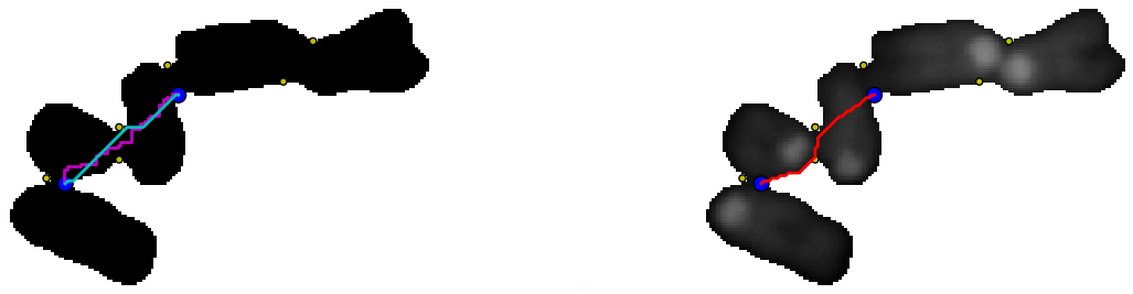
On the left, two paths (depending on the chosen pixel neighborhood) between the two blue points were overlaid on a binary image (background is set to 255 and the foreground to 0). The path were determined as follow using skimage 0.8dev:
graph.route_through_array(negbin ,p1,p2,fully_connected=False)
 or
 graph.route_through_array(negbin ,p1,p2,fully_connected=True)

  • negbin: the negative binary image
  • p1, p2: the two points figured in blue.

On the right the background (0) was set to 255 (white), the path (red) between the two points was determined by minimizing the "greyscale cost", that is through the valleys between the two points is the image is viewed as a greyscaled landscape.

All the paths can be determined (left), and then the paths can be sorted according to their cost (right). The four paths with the smallest cost are figured in red (left).


Download code.

or see bellow:


# -*- coding: utf-8 -*-
"""
Created on Tue Oct 23 08:06:37 2012
@author: Jean-Patrick
"""
import os
import numpy as np
import matplotlib.pyplot as plt
import skimage.io as sio
import skimage
#import skimage.viewer as viewer
#from skimage.draw import ellipse
from skimage import graph
from skimage.measure import find_contours, approximate_polygon, \
subdivide_polygon
import cmath
from math import pi
import itertools
def addpixelborder(im):
x,y = im.shape
dy = np.zeros((y,))
im = np.vstack((im,dy))
im = np.vstack((dy,im))
im = np.transpose(im)
x,y = im.shape
dy = np.zeros((y,))
im = np.vstack((im,dy))
im = np.vstack((dy,im))
im = np.transpose(im)
return im
def angle(p1,p2,p3):
'''get the angle between the vectors p2p1,p2p3 with p a point
'''
z1=complex(p1[0],p1[1])
z2=complex(p2[0],p2[1])
z3=complex(p3[0],p3[1])
v12=z1-z2
v32=z3-z2
#print v12,v32
angle=(180/pi)*cmath.phase(v32/v12)
return angle
def angleBetweenSegments(contour):
angles = []
points = list(contour)
points.pop()
#print 'contour in def',len(contour)
l = len(points)
for i in range(len(points)+1):
#print 'i',i,' i-1',i-1,' (i+1)%l',(i+1)%l
prv_point=points[(i-1)%l]
mid_point=points[i % l]
nex_point=points[(i+1)%l]
angles.append(angle(prv_point,mid_point,nex_point))
return angles
def get_polygon_single_closed_curve(image, tolerance):
contours_list = find_contours(image, 0.01)
p = subdivide_polygon(contours_list[0], degree=5, preserve_ends=True)
print 'sub polygon type', type(p)
coord = approximate_polygon(p, tolerance)
print 'approximate polygon', type(coord)
return coord
def get_polygon_from_single_open_curve(image,tolerance):
'''need to know where an axis is curved....
image: where we need an axis (black background)
'''
sk = skimage.morphology.medial_axis(im>0)
skel = skimage.img_as_int(sk)
tmp = np.where(skel>0)#tuple of x , y
image_to_points = np.vstack((tmp[0],tmp[1]))# array of [x,y]
#spoly = subdivide_polygon(image_to_points, degree=3, preserve_ends=True)
coord = approximate_polygon(image_to_points, tolerance=1.5)
return coord
def filter_angles(coordinates_list, angles_list, angle_min, angle_max):
table = np.array([coordinates_list[0][0],coordinates_list[0][1],angles_list[0]])
for i in range(len(angles_list[1:])):
current = np.array([coordinates_list[i][0],coordinates_list[i][1],angles_list[i]])
table = np.vstack((table,current))
filtered = table[(angle_max>table[:,2]) & (table[:,2]>angle_min)]
return filtered.astype(int)
def makePointsCombinations(pointsArray,p_elements):
''' an array has the form
li_i, col_i,angle_i
with 0<=i<=k-1. k points
'''
points=[]
k=pointsArray.shape[0]
for p in range(k):
lin = pointsArray[p][0]
col = pointsArray[p][1]
points.append((lin,col))
return itertools.combinations(points,p_elements)
def make_path(allcosts, index):
k = allcosts.keys()
k.sort()
# print k[0:4]
# print len(k),min(k),max(k)
x=[]
y=[]
for p in allcosts[k[index]]:
x.append(p[0])
y.append(p[1])
return x,y
if __name__ == "__main__":
user=os.path.expanduser("~")
workdir=os.path.join(user,"QFISH","JPPAnimal","JPP52","11","DAPI","particles")
image='part25.png'
complete_path=os.path.join(workdir,image)
im = sio.imread(complete_path)
im = addpixelborder(im)
im = np.uint8(im)
negbin = 255-np.uint(im>0)
walls = np.copy(im)
walls[walls == 0] = 255
coord2 = get_polygon_single_closed_curve(im, tolerance=3)
contours = find_contours(im, 0.1)
angles = angleBetweenSegments(coord2)
negative = filter_angles(coord2, angles,-165,-45)
positive = filter_angles(coord2, angles,50,130)
combinations = makePointsCombinations(negative,2)
allpaths = {}
allcosts = {}
for c in combinations:
p1 = np.asarray(c[0])
p2 = np.asarray(c[1])
#print p1,p2
g = graph.route_through_array(negbin ,p1,p2,fully_connected=True)
allpaths[c] = g
allcosts[g[1]] = g[0]
#==============================================================================
#
#==============================================================================
plt.subplot(321,frameon = False,xticks = [], yticks = [])
plt.imshow(im, interpolation='nearest', cmap=plt.cm.gray)
# plt.scatter(p1[1], p1[0], s=200, c='b')
# plt.scatter(p2[1], p2[0], s=200, c='b')
for n, contour in enumerate(contours):
plt.plot(contour[:, 1], contour[:, 0], linewidth=2)
plt.plot(coord2[:, 1], coord2[:, 0], linewidth=2, color='y')
for i in range(positive.shape[0]):
plt.scatter(positive[i][1], positive[i][0], s=100, c='r')
for i in range(negative.shape[0]):
plt.scatter(negative[i][1], negative[i][0], s=100, c='y')
#==============================================================================
#
#==============================================================================
plt.subplot(323,frameon = False,xticks = [], yticks = [])
p1=np.array([negative[7][0],negative[7][1]])
p2=np.array([negative[5][0],negative[5][1]])
mincost_n4 = graph.route_through_array(negbin ,p1,p2,fully_connected=False)
minpoints_n4=mincost_n4[0]
x4=[]
y4=[]
for p in minpoints_n4:
x4.append(p[0])
y4.append(p[1])
for i in range(negative.shape[0]):
plt.scatter(negative[i][1], negative[i][0], s=20, c='y')
mincost_n8 = graph.route_through_array(negbin ,p1,p2,fully_connected=True)
minpoints_n8=mincost_n8[0]
x8=[]
y8=[]
for p in minpoints_n8:
x8.append(p[0])
y8.append(p[1])
plt.scatter(p1[1], p1[0], s=100, c='b')
plt.scatter(p2[1], p2[0], s=100, c='b')
plt.plot(y4[:],x4[:], linewidth=2, c='m')
plt.plot(y8[:],x8[:], linewidth=2, c='c')
plt.imshow(negbin, interpolation='nearest', cmap=plt.cm.gray)
#==============================================================================
#
#==============================================================================
plt.subplot(324,frameon = False,xticks = [], yticks = [])
p1=np.array([negative[7][0],negative[7][1]])
p2=np.array([negative[5][0],negative[5][1]])
for i in range(negative.shape[0]):
plt.scatter(negative[i][1], negative[i][0], s=20, c='y')
mincost = graph.route_through_array(walls ,p1,p2,fully_connected=True)
minpoints=mincost[0]
x=[]
y=[]
for p in minpoints:
x.append(p[0])
y.append(p[1])
plt.scatter(p1[1], p1[0], s=100, c='b')
plt.scatter(p2[1], p2[0], s=100, c='b')
plt.plot(y[:],x[:], linewidth=2, c='r')
plt.imshow(walls, interpolation='nearest', cmap=plt.cm.gray)
#==============================================================================
#
#==============================================================================
plt.subplot(322,frameon = False,xticks = [], yticks = [])
copycomb = makePointsCombinations(np.copy(negative),2)
#print 'copycomb',copycomb.shape
xy = zip(*itertools.chain.from_iterable(copycomb))
#
plt.imshow(im, interpolation='nearest', cmap=plt.cm.gray)
plt.plot(xy[1],xy[0],color = 'brown', marker = 'o')
#==============================================================================
#
#==============================================================================
plt.subplot(325,frameon = False,xticks = [], yticks = [])
plt.imshow(im, interpolation='nearest', cmap=plt.cm.gray)
for i in range(len(allcosts)):
x,y =make_path(allcosts, i)
#print x,y
plt.plot(y[:],x[:], linewidth=1, c='c')
for i in range(negative.shape[0]):
plt.scatter(negative[i][1], negative[i][0], s=20, c='y')
costs = allcosts.keys()
costs.sort()
smallest = costs[0:4]
for cost in smallest:
current_path =allcosts[cost]
xy=np.asarray(current_path)
plt.plot(xy[:,1],xy[:,0], linewidth=2, c='r')
#==============================================================================
#
#==============================================================================
plt.subplot(326,frameon = True)
costs = allcosts.keys()
costs.sort()
plt.semilogy(range(len(costs)),costs[:], marker='o')
plt.xlabel('rank')
plt.ylabel('Grey level cost')
#p(lt.set_xlabel('rank')
#plt.set_ylabel('Grey level Cost')
#==============================================================================
#
#==============================================================================
plt.show()

Wednesday, October 24, 2012

Contour : looking for negatively curved domains

A contour was previously explored with the convexity defects  algorithm implemented in opencv. Some highly curved domains  failed to be detected because of the contour shape.
Curved domains missed by convexity defects detection

Using polygonal approximation imlemented in skimage 0.8 dev, positively curved domains as well as negatively curved domains on a contour can be sorted:
Contour of a chromosomes cluster (blue), polygonal approximation (yellow). Red points: positive curvature. Yellow points: negative curvature.

From a segmented particle, a polygonal approximation of the contour is extracted.
Points of the polygon are used to compute an angle between two consecutive vectors (Here using the complex affix of vectors):

Positive angles correspond to convex domains and negative angles to concave domains.


The code has to be modified to filter angles according to a given range. 

The code can be modified as follow to filter angles corresponding to curved domains:

  • positive = table[(135>table[:,2]) & (table[:,2]>45)]
  • negative = table[(-45>table[:,2]) & (table[:,2]>-135)]
Curved domains on polygonal approximation of a chromosomes cluster contour.

Download code


# -*- coding: utf-8 -*-
"""
Created on Tue Oct 23 08:06:37 2012
@author: Jean-Patrick
"""
import os
import numpy as np
import matplotlib.pyplot as plt
import skimage.io as sio
import skimage
import skimage.viewer as viewer
from skimage.draw import ellipse
from skimage.measure import find_contours, approximate_polygon, \
subdivide_polygon
import cmath
from math import pi
def addpixelborder(im):
x,y = im.shape
dy = np.zeros((y,))
im = np.vstack((im,dy))
im = np.vstack((dy,im))
im = np.transpose(im)
x,y = im.shape
dy = np.zeros((y,))
im = np.vstack((im,dy))
im = np.vstack((dy,im))
im = np.transpose(im)
return im
def angle(p1,p2,p3):
'''get the angle between the vectors p2p1,p2p3 with p a point
'''
z1=complex(p1[0],p1[1])
z2=complex(p2[0],p2[1])
z3=complex(p3[0],p3[1])
v12=z1-z2
v32=z3-z2
print v12,v32
angle=(180/pi)*cmath.phase(v32/v12)
return angle
def angleBetweenSegments(contour):
angles = []
points = list(contour)
points.pop()
#print 'contour in def',len(contour)
l = len(points)
for i in range(len(points)+1):
print 'i',i,' i-1',i-1,' (i+1)%l',(i+1)%l
prv_point=points[(i-1)%l]
mid_point=points[i % l]
nex_point=points[(i+1)%l]
angles.append(angle(prv_point,mid_point,nex_point))
return angles
user=os.path.expanduser("~")
workdir=os.path.join(user,"QFISH","JPPAnimal","JPP52","11","DAPI","particles")
image='part25.png'
complete_path=os.path.join(workdir,image)
#print complete_path
im = sio.imread(complete_path)
im = addpixelborder(im)
fig, ax1= plt.subplots(ncols=1, figsize=(9, 4))
contours = find_contours(im, 0.01)
print type(contours)
print len(contours)
p = subdivide_polygon(contours[0], degree=5, preserve_ends=True)
#print p
coord = approximate_polygon(p, tolerance=1.5)
coord2 = approximate_polygon(p, tolerance=2)
print coord2[-1]
print coord2[0]
print coord2[1]
print 'coord',type(coord2[0])
ax1.imshow(im, interpolation='nearest', cmap=plt.cm.gray)
#plt.imshow(im, interpolation='nearest')
contour0=contours[0]
pf=contours[-1]
print 'contc',contour0[0]
angles = angleBetweenSegments(coord2)
table = np.array([coord2[0][0],coord2[0][1],angles[0]])
for i in range(len(angles[1:])):
current = np.array([coord2[i][0],coord2[i][1],angles[i]])
table = np.vstack((table,current))
positive = table[table[:,2]>0]
negative = table[table[:,2]<0]
for n, contour in enumerate(contours):
ax1.plot(contour[:, 1], contour[:, 0], linewidth=4)
ax1.plot(coord[:, 1], coord[:, 0], linewidth=1, color='r')
ax1.plot(coord2[:, 1], coord2[:, 0], linewidth=1, color='y')
ax1.scatter(contour0[0][1],contour0[0][0],s=150, c='m',marker='o')
ax1.scatter(pf[0][1],pf[0][0],s=150, c='y',marker='*')
for i in range(positive.shape[0]):
ax1.scatter(positive[i][1], positive[i][0], s=200, c='r')
for i in range(negative.shape[0]):
ax1.scatter(negative[i][1], negative[i][0], s=200, c='y')
plt.show()
#
#views = viewer.CollectionViewer((im))
#views.show()