MFISH dataset available .

MFISH dataset from Wade Schwartzkoptf is available here.

Build Mamba 1.0 on Ubuntu 10.10

Mamba is a python mathematical morphology library. When dependencies are satisfied, installation is fast and simple. Once installed, from a python console:

>>> import mamba

>>> dir(mamba) 

['DEFAULT_GRID', 'EMPTY', 'FILLED', 'HEXAGONAL', 'MambaError', 'SQUARE', 'VERSION', '__builtins__', '__doc__', '__file__', '__name__', '__package__', '_always_show', '_blue_val', '_edge', '_green_val', '_grid', '_i', '_image_index', '_j', '_k', '_red_val', 'add', 'addConst', 'basinSegment', 'buildNeighbor', 'checkEmptiness', 'compare', 'computeDistance', 'computeMaxRange', 'computeRange', 'computeVolume', 'convert', 'convertByMask', 'copy', 'copyBitPlane', 'copyBytePlane', 'copyLine', 'cropCopy', 'diff', 'diffNeighbor', 'divConst', 'dualbuildNeighbor', 'extractFrame', 'generateSupMask', 'getDirections', 'getDisplayer', 'getHistogram', 'getImageCounter', 'getShowImages', 'gridNeighbors', 'hierarBuild', 'hierarDualBuild', 'hitOrMiss', 'imageMb', 'infFarNeighbor', 'infNeighbor', 'inverted_rainbow', 'label', 'logic', 'lookup', 'mambaCore', 'mbUtls', 'mul', 'mulConst', 'negate', 'os', 'patchwork', 'rainbow', 'raiseExceptionOnError', 'raiseWarning', 'rotateDirection', 'setDefaultGrid', 'setImageIndex', 'setMaxDisplay', 'setMinDisplay', 'setShowImages', 'shift', 'sub', 'subConst', 'supFarNeighbor', 'supNeighbor', 'threshold', 'tidyDisplays', 'transposeDirection', 'watershedSegment']

Classifying chromosomes with scikit-learn

A trained dataset was build from 5 metaphases corresponding to 205 classified chromosomes or nuclei falling in one of four categories: single chromosome, overlapping chromosomes, nuclei or dusts(artefact of image segmentation).  

Two features were chosen to classify the particles:

• The particle area (normalised by image size)
• The convex-hull area of the particle ( area/convex hull). The idea is that particles that are clustered chromosomes will have a smaller ratio than single chromosomes.

The trained dataset is used to recognise 49 particles segmented from a sixth metaphase and then the predictions from the classifier compared to hand classified particles reached...

                                                             59.18%

# -*- coding: utf-8 -*-
"""
Created on Fri Oct  7 13:08:57 2011

@author: Jean-Patrick Pommier
"""
import KarIO
import os
import pylab
import pandas
import numpy as np
from sklearn import svm
#make a configurator object
config=KarIO.ClassifConf()
#build the the name feature file
##list all the feature files
##répertoire courant : os.listdir(os.getcwd())
featurespath=os.path.join(os.getcwd(),"Results","features")
labelpath=os.path.join(os.getcwd(),"Results","labels")
#print featurespath
##open features csv files
featuresFilesList=os.listdir(featurespath)
labelsFilesList=os.listdir(labelpath)
##
metalist=[0,1,2,3,4]
def makeDataShape(meta):
    featfile=config.user+'-'+config.slide+'-'+config.metaphases_list[meta]+'-'+config.counterstain+'.csv'
    labelfile='shapeCateg-'+featfile
    fea=pandas.read_csv(os.path.join(featurespath,featfile),header=None,index_col=None,names=['particle','ratio','area'])
    lab=pandas.read_csv(os.path.join(labelpath,labelfile),header=None,index_col=None,names=['particle','type'])
    del lab['particle']    
    #merge columns:features and label
    data=fea.join(lab)
    data.insert(0,'meta',int(config.metaphases_list[meta]))
    #print data
    return data

bigdata=makeDataShape(0)
for meta in metalist:
    bigdata=bigdata.append(makeDataShape(meta),ignore_index=True)

single=bigdata[bigdata['type']=='single']
touching=bigdata[bigdata['type']=='touching']
nuclei=bigdata[bigdata['type']=='nuclei']
dusts=bigdata[bigdata['type']=='dusts']

##ploting with pylab
#different colors according to the category

fig=pylab.figure()
ax = fig.add_subplot(111)
ax.scatter(single['ratio'],single['area'],c='green',marker='o')
ax.scatter(touching['ratio'],touching['area'],c='red',marker='o')
ax.scatter(nuclei['ratio'],nuclei['area'],c='blue',marker='o')
ax.scatter(dusts['ratio'],dusts['area'],c='pink',marker='o')

#train a classifier
trainedData=bigdata[bigdata['meta']<15]
untrained=bigdata[bigdata['meta']>=15]
print 'trained data'
print trainedData[:5]
#extract two columns from trainedData
#convert to numpy array
features=trainedData.ix[:,['ratio','area']].as_matrix(['ratio','area'])
test_features=untrained.ix[:,['ratio','area']].as_matrix(['ratio','area'])
print 'features'
print features[:5]
print 'features shape',features.shape
print 'features type',type(features)
##label is a string:single, touching,nuclei,dust
print 'labels convertion'
lab1=trainedData['type']
print 'lab1',type(lab1)
f=pandas.Factor(lab1)
print 'factor f',type(f)
print 'labels',f.labels[:5]
print 'labels type',type(f.labels)
print 'labels shape',f.labels.shape
#
##Classify with sklearn
classifier = svm.SVC()
model = classifier.fit(features,f.labels)
predicted=classifier.predict(test_features)

#match predicted /classified
hiddenlab1=untrained['type']
hiddf=pandas.Factor(hiddenlab1)
match=(predicted==hiddf.labels)
print"prediction"
print predicted[:5]
print 'true classification'
print hiddf.labels[:5]
print 'match'
print match[:5]
##Count sucess
success=np.sum(match[:]==True)
rate=100.0*success/(1.0*len(match))
print 'rate of good classification',success,'out of',len(match),'particles'
print rate,'% success'

chromosome classification:workflow

The work-flow from raw DAPI image to two features scatter plot can be summarised as follow:

Yellow:to be written

Combining five metaphases, with two features (the area of the segmented particles and the ratio between the particle area and the area of convex hull of the particle) yields the following scatter plot where three clusters can be distinguished:

• blue cluster: nuclei
• red cluster: overlapping chromosomes
• green cluster:single chromosomes
• pink cluster:particles resulting from segmentation artefacts, some corresponds to nuclei touching the image border and should have been classified as nuclei.

As seen in the previous post the green and red clusters partially overlap. The graphic was build as follow with pandas (with some help):

import KarIO
import os,csv
import pylab
import pandas
#make a configurator object
config=KarIO.ClassifConf()
#build the the name feature file
##list all the feature files
##répertoire courant : os.listdir(os.getcwd())
featurespath=os.path.join(os.getcwd(),"Results","features")
labelpath=os.path.join(os.getcwd(),"Results","labels")
#print featurespath
##open features csv files
featuresFilesList=os.listdir(featurespath)
labelsFilesList=os.listdir(labelpath)
##
metalist=[0,1,2,3,4]
#metaphase=2
def makeDataShape(meta):
    featfile=config.user+'-'+config.slide+'-'+config.metaphases_list[meta]+'-'+config.counterstain+'.csv'
    labelfile='shapeCateg-'+featfile
    fea=pandas.read_csv(os.path.join(featurespath,featfile),header=None,index_col=None,names=['particle','ratio','area'])
    lab=pandas.read_csv(os.path.join(labelpath,labelfile),header=None,index_col=None,names=['particle','type'])
    del lab['particle']    
    #merge columns:features and label
    data=fea.join(lab)
    data.insert(0,'meta',config.metaphases_list[meta])
    #print data
    return data
bigdata=makeDataShape(0)
for meta in metalist:
    bigdata=bigdata.append(makeDataShape(meta),ignore_index=True)
single=bigdata[bigdata['type']=='single']
touching=bigdata[bigdata['type']=='touching']
nuclei=bigdata[bigdata['type']=='nuclei']
dusts=bigdata[bigdata['type']=='dusts']
##ploting with pylab
#different colors according to the category
fig=pylab.figure()
ax = fig.add_subplot(111)
ax.scatter(single['ratio'],single['area'],c='green',marker='o')
ax.scatter(touching['ratio'],touching['area'],c='red',marker='o')
ax.scatter(nuclei['ratio'],nuclei['area'],c='blue',marker='o')
ax.scatter(dusts['ratio'],dusts['area'],c='pink',marker='o')
pylab.show()

chromosomes, overlapping chromosomes and nuclei

In an attempt to find features to distinguish chromosomes from overlapping chromosomes or from nuclei or small image segmentation artifacts ("dusts"), the area and the convex-hull area of isolated particles were computed after segmentation of a metaphasic chromosome image.

Image segmentation and convex-hull area computation were performed with scripts written previously. The features were saved in csv files.

miniKar produced an other csv file where the particle category (label) was saved.

This is an opportunity to handle the data with the pandas library and to see from this limited data set if the two features may be good candidates to classify at least particles in one of the three categories (single, overlapping, nuclei). A features file and the labels file were loaded, merged in one data frame. The features were filtered according to the label (the particle category) and then were displayed in a scatter plot:

green:single chromosomes; red overlapping chromosomes; blue:nuclei

The normalized area is the 1000*area of a particle divided by the image size (1024x1536). From this scatter plot, it's clear that at least an other feature will be necessary to separate the single chromosomes from the overlapping chromosomes. This may be due to the chromosomes bending.

A surprising thing, the ratio should be such: area/convexhull <1 and it is not true for all the particles.

import KarIO
import os,csv
import pylab
import pandas
#make a configurator object
config=KarIO.ClassifConf()
#build the the name feature file
##list all the feature files
##répertoire courant : os.listdir(os.getcwd())
featurespath=os.path.join(os.getcwd(),"Results","features")
labelpath=os.path.join(os.getcwd(),"Results","labels")
#print featurespath
##open features csv files
featuresFilesList=os.listdir(featurespath)
labelsFilesList=os.listdir(labelpath)
##
#let's find a pair of feature file/label file
#open with pandas
#two files match if they come from the same metaphase

featfile=config.user+'-'+config.slide+'-'+config.metaphases_list[2]+'-'+config.counterstain+'.csv'
labelfile='shapeCateg-'+featfile

fea=pandas.read_csv(os.path.join(featurespath,featfile),header=None,names=['particle','ratio','area'])
lab=pandas.read_csv(os.path.join(labelpath,labelfile),header=None,names=['particle','type'])
#merge columns:features and label
data=fea.join(lab)
single=data[data['type']=='single']
touching=data[data['type']=='touching']
nuclei=data[data['type']=='nuclei']
dusts=data[data['type']=='dusts']

##ploting with pylab
#different colors according to the category

fig=pylab.figure()
ax = fig.add_subplot(111)
ax.scatter(single['ratio'],single['area'],c='green',marker='o')
ax.scatter(touching['ratio'],touching['area'],c='red',marker='o')
ax.scatter(nuclei['ratio'],nuclei['area'],c='blue',marker='o')
pylab.show()

making a scatter plot with tags: playing with the iris data set

I need to display a scatterplot and to distinguish the points according to a category. I start with the iris dataset available in scikit-learn:

# -*- coding: utf-8 -*-
"""
"""
import pylab
from scikits.learn import datasets
iris = datasets.load_iris()
X=iris.data
Y=iris.target
print X
fig=pylab.figure()
ax = fig.add_subplot(111, aspect='equal')
print type(iris)
print iris.data.shape
print X[0:4,1]
print X[0:4,2]
print Y[0:4]
ax.scatter(X[:,0],X[:,1],c=Y[:])
pylab.show()

The Y column contains the labels stored as numerical values used to select the a color.

Chromosomes classification with a configurable pygame script :miniKar.py

 

Up to now miniKar doesn't recognize chromosomes. It is used to build a training set for :

• supervised learning.
• features selection

miniKar can be configured with a configuration file which specify the path to the chromosomes images and the categories of of the training set (but also the size and positions of the red areas, representing the categories).

#read by miniChromClassif.py
[Fluorochromes]
Counter_stain=DAPI
Probes=Cy3,Cy5,FITC
[Images Path]
work_dir=/home/claire/Applications/ImagesTest/
user=jp
slide=Jpp48
field_list=13,14
[ClassifierGUI]
screen_size=1024,768
categories_number=4
categories_list=single chr,touching chr,nuclei,dusts
box_size=240,380
#((col,li),(col+200+30,li),...)!!
box_position=(20,300),(268,300),(516,300),(764,300)

From left to right, the red areas represents

• the single chromosomes.
• the overlapping chromosomes
• the nuclei
• dusts (or segmentation artifacts)

By varying, the number of categories, it is already possible to perform by hand, a real karyotyping, even there is no tool to resolve overlapping chromosomes.

To use miniKar, three files must be in the same directory:

• configuration.cfg

• KarIO.py
• miniKar

Suppose we want to classify the following particles into one of the four categories:

1. single chromosome
2. touching chromosomes
3. nuclei
4. dust

First download a chromosome dataset  then store it somewhere. On a ubuntu/linux the path to the images may be :

/home/user/cytogenetic_images/project/exampleslide/metaphase/DAPI/particles

Modify the configuration.cfg file to fit the path, for example:

work_dir=/home/user/cytogenetic_images
user=project
slide=exampleslide
field_list=1

Run minikar.py from a console by : python minikar01.py or from your favorite IDE (spyder, ninja-ide,...). Something like this should be visible:

The green background is uggly, but the small things are visible. After having classified the different chromosomes, one can have :

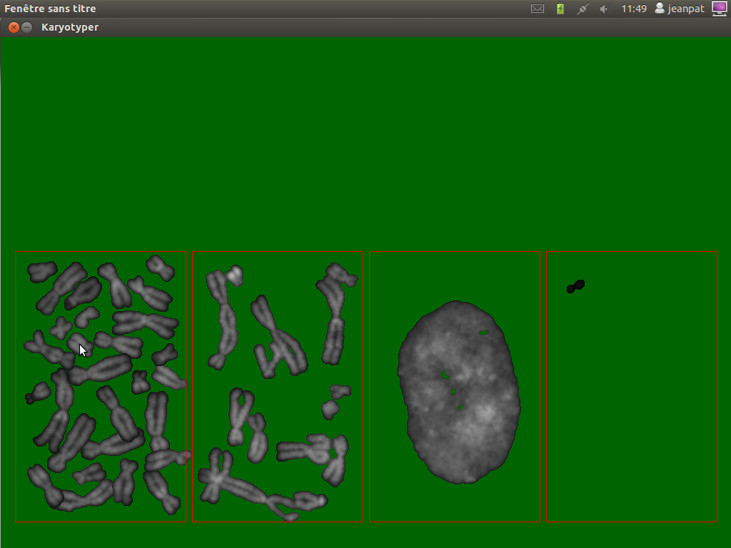
On pressing  the keyboard Esc,  minikar save a first file which associes the file name of a particle and its category and produce a second one in the csv format.
To classify the chromosomes from several  metaphases, the configuration.cfg file must be modified for each metaphase:

field_list=1

To classify the metaphase 13 in the folder exampleslide , modify the file as:

 field_list=13

If features are computed for each particle, then they can be associated to a category for further processing with a classifier. Here, chromosomes from 14 metaphases were classified, five features related to the convex hull were used.