Which structuring elements to detect branched points?

In a 2D skeleton obtained after thinning of a binary image, pixels having 3 or 4 (or more...) neighbors are branched-points. Hit-or-miss operator can be used to detect branched points (or junction points). Structuring elements, SE, can be 3x3 arrays representing the pixels configuration to be detected. Here different 3x3 structuring elements were explored on some simple test images with the hit-or-miss operator implemented in mahotas 1.0 .

• There are two SE to detect pixels with 4 neighbors, called here X0 and X1.
• There are two set of SE detecting pixels with at least 3 pixels, a Y-like configuration and a T-like configuration. Each of these configurations can be rotated by 45°, making 16 different SE.

18 SE were found , since don't care pixels were used a branched points can be detected by different SE, a pixel detected by X0 should be detected by T4 too. The 18 SE can be displayed as 3x3 image:

Black:background pixel (0), Blue: foreground pixel (1), Red:Don't care pixel (0 or 1)

Applied on a small skeleton-like test image (left), two branched-points  (junction) and four end-points are detected:

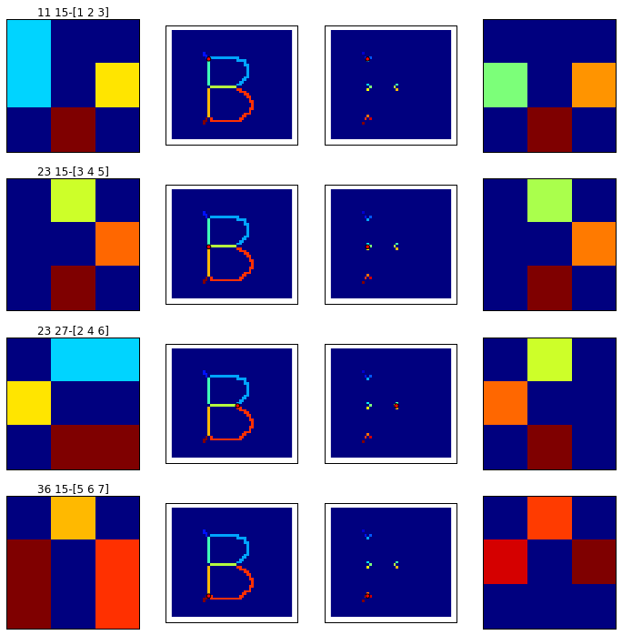
On a larger image, from the SIID images database:

Hit-or-miss transformation applied on the skeleton (up right), yields end-points (lower right). Since the same branched-points can be detected by different structuring elements, branched points appear of a variable color according to the detection occurence. Moreoever, branched-points can be connected yielding a branched domain of pixels.

ipython notebook

HMT-SE.ipynb

From binary image skeleton to networkx graph.

To recognize objects in an image methods involving graphs have been developped as the shock graph method. These graphs are derived from image skeleton and then handled, compared. However, it seems taken for granted that a graph is available for work.

Here is proposed a python code generating a networkx graph object from the skeleton of a binary image.

The image of the B letter was chosen as model. The image is generated with PIL:

Skeleton decomposition:

The shape skeleton is computed by morphological thining, branched points are extracted from the skeleton with a hit-or-miss operator and labelled:

Finding the neighborhood of the branched points:

• The end points are extracted and labelled from the initial skeleton (top left image) .

• The edges are obtained by difference between the skeleton of the shape and the branched points of the skeleton. Seven edges were found and labelled from 1 to 7 (middle left image).

• The edges are pruned by one pixel, the labels values are 1,2,3,4,5,6,7 (middle right image).

• The edges end points are then extracted and labelled individually (1,2,3,...,14) (bottom left image).

• The end points are also labelled according to their edge of origin ( 1,2,3,4,5,6,7), (bottom right image).

For each branched point, its neighborhood is isolated to get the labels of the adjacent end points (right images):

Building the graph:

The graph is build by adding branched points first (vertex 1, 2, 3, 4), it assumes that at least one branched point exists, then  end points adjacent to the branched points are added (vertex 8,9,10 and 11,12,13 and 14,15,16): 

The remaining lonely end points are added to the graph (vertex 17, 18):

The end points are linked using the pruned edges, the edges are weighted according to their pixel size:

Graph of the letter B, without initial skeleton pruning. The edges length here do not match to their weight

A bug somewhere (update fri 06, 2013):

For some shapes, as 'Y':

The algorithm fails at the end points linking step. A way to cure the situation is to prune the initial skeleton of 'Y' once:

 

In the case of the letter 'A', the skeleton must be pruned three times for the algorithm to succeed:

Bug origin:

With the letter 'Y', with initial skeleton pruning, the algorithm yields the following graph:

Branched points are figured in red circles on the image of labelled edges and end points are figured by a white star.

In the case of the letter 'A', the algorithm yields :

The bug seems to come from too short edges as after three pruning steps removing the small barbs on the top of the letter, the algorithm succeeds in producing a graph

Download ipython notebook

 ipython notebook available at ipython.org
or from gist:

Loading

Sorry, something went wrong. Reload?

Sorry, we cannot display this file.

Sorry, this file is invalid so it cannot be displayed.

view raw SkeletonToGraph.ipynb hosted with ❤ by GitHub

	# -*- coding: utf-8 -*-
	# <nbformat>3.0</nbformat>
	# <codecell>
	import Image, ImageDraw, ImageFont
	import mahotas as mh
	from mahotas import polygon
	import pymorph as pm
	import networkx as nx
	from scipy import ndimage as nd
	import skimage.transform as transform
	import skimage.io as sio
	import scipy.misc as sm
	import os
	import math
	# <codecell>
	def branchedPoints(skel):
	branch1=np.array([[2, 1, 2], [1, 1, 1], [2, 2, 2]])
	branch2=np.array([[1, 2, 1], [2, 1, 2], [1, 2, 1]])
	branch3=np.array([[1, 2, 1], [2, 1, 2], [1, 2, 2]])
	branch4=np.array([[2, 1, 2], [1, 1, 2], [2, 1, 2]])
	branch5=np.array([[1, 2, 2], [2, 1, 2], [1, 2, 1]])
	branch6=np.array([[2, 2, 2], [1, 1, 1], [2, 1, 2]])
	branch7=np.array([[2, 2, 1], [2, 1, 2], [1, 2, 1]])
	branch8=np.array([[2, 1, 2], [2, 1, 1], [2, 1, 2]])
	branch9=np.array([[1, 2, 1], [2, 1, 2], [2, 2, 1]])
	br1=mh.morph.hitmiss(skel,branch1)
	br2=mh.morph.hitmiss(skel,branch2)
	br3=mh.morph.hitmiss(skel,branch3)
	br4=mh.morph.hitmiss(skel,branch4)
	br5=mh.morph.hitmiss(skel,branch5)
	br6=mh.morph.hitmiss(skel,branch6)
	br7=mh.morph.hitmiss(skel,branch7)
	br8=mh.morph.hitmiss(skel,branch8)
	br9=mh.morph.hitmiss(skel,branch9)
	return br1+br2+br3+br4+br5+br6+br7+br8+br9
	def endPoints(skel):
	endpoint1=np.array([[0, 0, 0],
	[0, 1, 0],
	[2, 1, 2]])
	endpoint2=np.array([[0, 0, 0],
	[0, 1, 2],
	[0, 2, 1]])
	endpoint3=np.array([[0, 0, 2],
	[0, 1, 1],
	[0, 0, 2]])
	endpoint4=np.array([[0, 2, 1],
	[0, 1, 2],
	[0, 0, 0]])
	endpoint5=np.array([[2, 1, 2],
	[0, 1, 0],
	[0, 0, 0]])
	endpoint6=np.array([[1, 2, 0],
	[2, 1, 0],
	[0, 0, 0]])
	endpoint7=np.array([[2, 0, 0],
	[1, 1, 0],
	[2, 0, 0]])
	endpoint8=np.array([[0, 0, 0],
	[2, 1, 0],
	[1, 2, 0]])
	ep1=mh.morph.hitmiss(skel,endpoint1)
	ep2=mh.morph.hitmiss(skel,endpoint2)
	ep3=mh.morph.hitmiss(skel,endpoint3)
	ep4=mh.morph.hitmiss(skel,endpoint4)
	ep5=mh.morph.hitmiss(skel,endpoint5)
	ep6=mh.morph.hitmiss(skel,endpoint6)
	ep7=mh.morph.hitmiss(skel,endpoint7)
	ep8=mh.morph.hitmiss(skel,endpoint8)
	ep = ep1+ep2+ep3+ep4+ep5+ep6+ep7+ep8
	return ep
	def pruning(skeleton, size):
	'''remove iteratively end points "size"
	times from the skeleton
	'''
	for i in range(0, size):
	endpoints = endPoints(skeleton)
	endpoints = np.logical_not(endpoints)
	skeleton = np.logical_and(skeleton,endpoints)
	return skeleton
	# <codecell>
	image = Image.new("RGBA", (600,150), (255,255,255))
	draw = ImageDraw.Draw(image)
	fontsize = 150
	font = ImageFont.truetype("/usr/share/fonts/truetype/liberation/LiberationMono-Regular.ttf", fontsize)
	txt = 'A'
	draw.text((30, 5), txt, (0,0,0), font=font)
	img = image.resize((188,45), Image.ANTIALIAS)
	plt.imshow(img)
	# <codecell>
	img = np.array(img)
	im = img[:,0:50,0]
	im = im < 128
	skel = mh.thin(im)
	# To fix the algorithm, prune the skeleton 1,2,3...
	skel = pruning(skel,3)
	bp = branchedPoints(skel)
	ep = endPoints(skel)
	edge = skel-bp
	edge_lab,n = mh.label(edge)
	bp_lab,_ = mh.label(bp)
	ep_lab,_ = mh.label(ep)
	# <codecell>
	figsize(10,20)
	subplot(141,frameon = False, xticks = [], yticks = [])
	title('pruning 0')
	imshow(mh.thin(im),interpolation = 'nearest')
	subplot(142,frameon = False, xticks = [], yticks = [])
	title('pruning 1')
	imshow(pruning(mh.thin(im),1),interpolation = 'nearest')
	subplot(143,frameon = False, xticks = [], yticks = [])
	title('pruning 2')
	imshow(pruning(mh.thin(im),2),interpolation = 'nearest')
	subplot(144,frameon = False, xticks = [], yticks = [])
	title('pruning 3')
	imshow(pruning(mh.thin(im),3),interpolation = 'nearest')
	# <codecell>
	subplot(221,frameon = False, xticks = [], yticks = [])
	title('skeleton')
	imshow(skel,interpolation = 'nearest')
	subplot(223,frameon = False, xticks = [], yticks = [])
	title('skel-bp -> label')
	imshow(edge_lab,interpolation = 'nearest')
	subplot(224,frameon = False, xticks = [], yticks = [])
	title('skel -> end points')
	imshow(ep_lab,interpolation = 'nearest')
	subplot(222,frameon = False, xticks = [], yticks = [])
	title('branched points (bp)')
	imshow(bp_lab,interpolation = 'nearest')
	# <codecell>
	endpoints = np.zeros(skel.shape)
	edges = np.zeros(skel.shape)
	for l in range(1,n+1):
	cur_edge = edge_lab == l
	cur_end_points = endPoints(cur_edge)
	pruned_edge = pruning(cur_edge,1)
	edges = np.logical_or(pruned_edge, edges)
	endpoints = np.logical_or(endpoints,cur_end_points)
	lab_bp, nbp = mh.label(bp)
	lab_ep, nep = mh.label(endpoints+ep)
	pruned_edges, ned = mh.label(edges)
	# <codecell>
	plt.figsize(13,8)
	subplot(321,frameon = False, xticks = [], yticks = [])
	title(str(np.unique(skel)))
	imshow(skel, interpolation='nearest')
	subplot(322,frameon = False, xticks = [], yticks = [])
	title(str(np.unique(lab_bp)))
	imshow(lab_bp, interpolation='nearest')
	subplot(323,frameon = False, xticks = [], yticks = [])
	title(str(np.unique(edge_lab)))
	imshow(edge_lab, interpolation='nearest')
	subplot(326,frameon = False, xticks = [], yticks = [])
	edge_mask = lab_ep>0
	ep_edgelab = edge_lab*edge_mask
	title(str(np.unique(ep_edgelab)))
	imshow(ep_edgelab,interpolation='nearest')#lab_ep
	subplot(324,frameon = False, xticks = [], yticks = [])
	title(str(np.unique(pruned_edges)))
	imshow(pruned_edges, interpolation='nearest')
	subplot(325,frameon = False, xticks = [], yticks = [])
	title(str(np.unique(lab_ep)))
	imshow(lab_ep, interpolation='nearest')
	# <headingcell level=3>
	# First make vertex from branched points and then link to the neighbouring endpoints
	# <codecell>
	BPlabel=np.unique(lab_bp)[1:]
	EPlabel=np.unique(lab_ep)[1:]
	EDlabel=np.unique(pruned_edges)[1:]
	G=nx.Graph()
	node_index=BPlabel.max()
	selected_ep_labels = []
	for bpl in BPlabel:
	#branched point location
	bp_row,bp_col= np.where(lab_bp==bpl)[0][0], np.where(lab_bp==bpl)[1][0]
	bp_neighbor= lab_ep[bp_row-1:bp_row+2,bp_col-1:bp_col+2]
	G.add_node(bpl,kind='BP',row=bp_row,col=bp_col,label=bpl)
	#branched point neighborhood
	neig_in_EP=lab_ep[bp_row-1:bp_row+2,bp_col-1:bp_col+2]
	neig_inEplabel=np.unique(neig_in_EP)[1:]
	print 'bp label',bpl,' pos',(bp_row,bp_col), 'ep neighbor label:',neig_inEplabel
	for epl in neig_inEplabel:
	selected_ep_labels.append(epl)
	node_index = node_index+1
	#print 'bp label',bpl,' pos',(bp_row,bp_col),neig_inEplabel, 'current ep',epl
	ep_row,ep_col= np.where(lab_ep==epl)[0][0], np.where(lab_ep==epl)[1][0]
	G.add_node(node_index,kind='EP',row=ep_row,col=ep_col,label=epl)
	G.add_edge(bpl,node_index, weight=1)
	print 'bp label',bpl,':',(bp_row,bp_col),neig_inEplabel,' -ep',epl,'(',node_index,')',':',(ep_row,ep_col),
	#print 'edge',(bpl, node_index)
	# <codecell>
	figsize(5,7)
	nx.draw(G)
	# <codecell>
	#Add isolated endpoints in the Graph
	#label of isolated end points
	lonely_ep = list(set(EPlabel) - set(selected_ep_labels))
	#lep:lonely ep
	for lep in lonely_ep:
	lep_row,lep_col= np.where(lab_ep==lep)[0][0], np.where(lab_ep==lep)[1][0]
	node_index = node_index+1
	G.add_node(node_index,kind='EP',row=lep_row,col=lep_col,label=lep)
	#print G.node[1]
	#edges dict
	edges={}
	for ed in EDlabel:
	edges[ed] = np.where(pruned_edges==ed),np.sum(pruned_edges==ed)
	#print edges[ed]
	#get nodes of kind EP
	ep_nodes=[node for node,data in G.nodes(data=True) if data['kind'] == 'EP']
	print ep_nodes
	#print edges.keys()
	ep_edges_lab = (lab_ep>0)*edge_lab
	#print G.nodes()
	#
	# <codecell>
	figsize(5,8)
	title('Isolated endpoints are added')
	nx.draw(G)
	# <headingcell level=3>
	# each endpoints pairs are linked
	# <codecell>
	# get all nodes of kind EP
	#get their label
	node_to_label={}
	label_to_node={}
	for node,data in G.nodes(data=True):
	if data['kind']=='EP':
	#print node,data['label']
	label_to_node[data['label']]=node
	print label_to_node
	# <codecell>
	#ep_labels from edge lab -> ep labels directly!
	#
	# node_index is not endpoint label!
	#
	map_epEdlab_epPair={}
	print EDlabel
	##plt.figsize(14,8)
	for elab in EDlabel:
	#subplot(3,3,elab)
	mask = (ep_edges_lab==elab)# ep lab=edges lab
	nodes_pair = np.unique(mask*lab_ep)[1:]
	pair_weight = np.sum(pruned_edges==elab)
	edge_image = (pruned_edges==elab)*elab
	print 'edge lab',elab, 'ep2 lab',nodes_pair,'weight',pair_weight,'node1:',nodes_pair[0]
	##title(str(elab)+str(np.where(ep_edgelab==elab))+str(nodes_pair))
	##imshow(mask, interpolation='nearest')
	node1 = label_to_node[nodes_pair[0]]
	node2 = label_to_node[nodes_pair[1]]
	G.add_edge(node1, node2, weight = pair_weight, image=edge_image)
	# <codecell>
	plt.figsize(5,8)
	pos=nx.spring_layout(G)
	#nx.draw_circular(G)
	#subplot(121)
	#nx.draw(G, width=range(1,4))
	#imshow(edge_lab,interpolation='nearest')
	#subplot(122)
	edge_labels=dict([((u,v,),d['weight']) for u,v,d in G.edges(data=True)])
	nx.draw(G)
	#nx.draw_networkx_edge_labels(G,pos,edge_labels=edge_labels)
	# <codecell>

view raw SkeletonToGraph.py hosted with ❤ by GitHub