Tuesday, August 20, 2013

Moving chromosomes with kivy

A demo application available with kivy, was modified to move chromosomes:

The application depends on two files: pictures.py and pictures.kv. Both files are in the same folder:
the particles folder contains the images to load.

The application should be modified so that the same zoom should be applied to all the chromosomes.

Update (22/08/2013) :

Independant zooming of the different chromosome images can be disabled.

Friday, August 16, 2013

Resolving overlapping chromosomes: an emblematic case

Metaphasic chromosomes preparations contain most of the time overlapping chromosomes as follow :
A cluster of two overlapping chromosomes
Here a cluster of two chromosomes was isolated and the two chromosomes were segmented using a contour based method implemented in an ipython notebook.
First a polygonal approximation of the contour is performed and negative corners are extracted as previously:

Polygonal approximation of the cluster contour (red line). Negative corners (yellow dots), positive corners (red dots).
Four points (the yellow ones) are then used to define a quadrilateral of maximal area:
The quadrilateral is converted to an image (overlapp domain:right image) and substracted from the original thresholded image yielding here four chromosomal elements (left image):
The four chromosomal elements are labelled:
Left:labelled chromosomal elements (the size is figured above the image). Right: labelled overlapping domain.
and isolated:
The idea is to used combinations of elements to build candidate chromosomes. Here the image is supposed to contain two chromosomes, so combinations of two elements in a set of four elements yield the following candidates:
For each candidate, several descriptors are computed: the number of connected components (cc), the eccentricity (ecc), the ratio chromosome area over its convex hull area (r) and the number of negative corner on the contour.
The two first highest ratio correspond to the two overlapping chromosomes which can be isolated:

Download the ipython notebook from google drive

Thursday, June 20, 2013

Which structuring elements to detect branched points?

In a 2D skeleton obtained after thinning of a binary image, pixels having 3 or 4 (or more...) neighbors are branched-points. Hit-or-miss operator can be used to detect branched points (or junction points). Structuring elements, SE, can be 3x3 arrays representing the pixels configuration to be detected. Here different 3x3 structuring elements were explored on some simple test images with the hit-or-miss operator implemented in mahotas 1.0 .
  • There are two SE to detect pixels with 4 neighbors, called here X0 and X1.
  • There are two set of SE detecting pixels with at least 3 pixels, a Y-like configuration and a T-like configuration. Each of these configurations can be rotated by 45°, making 16 different SE.
18 SE were found , since don't care pixels were used a branched points can be detected by different SE, a pixel detected by X0 should be detected by T4 too. The 18 SE can be displayed as 3x3 image:
Black:background pixel (0), Blue: foreground pixel (1), Red:Don't care pixel (0 or 1)
Applied on a small skeleton-like test image (left), two branched-points  (junction) and four end-points are detected:
On a larger image, from the SIID images database:
Hit-or-miss transformation applied on the skeleton (up right), yields end-points (lower right). Since the same branched-points can be detected by different structuring elements, branched points appear of a variable color according to the detection occurence. Moreoever, branched-points can be connected yielding a branched domain of pixels.

ipython notebook

HMT-SE.ipynb

Wednesday, June 5, 2013

From binary image skeleton to networkx graph.

To recognize objects in an image methods involving graphs have been developped as the shock graph method. These graphs are derived from image skeleton and then handled, compared. However, it seems taken for granted that a graph is available for work.
Here is proposed a python code generating a networkx graph object from the skeleton of a binary image.

The image of the B letter was chosen as model. The image is generated with PIL:

Skeleton decomposition:

The shape skeleton is computed by morphological thining, branched points are extracted from the skeleton with a hit-or-miss operator and labelled:

Finding the neighborhood of the branched points:

  • The end points are extracted and labelled from the initial skeleton (top left image) .
  • The edges are obtained by difference between the skeleton of the shape and the branched points of the skeleton. Seven edges were found and labelled from 1 to 7 (middle left image).
  • The edges are pruned by one pixel, the labels values are 1,2,3,4,5,6,7 (middle right image).
  • The edges end points are then extracted and labelled individually (1,2,3,...,14) (bottom left image).
  • The end points are also labelled according to their edge of origin ( 1,2,3,4,5,6,7), (bottom right image).
For each branched point, its neighborhood is isolated to get the labels of the adjacent end points (right images):

Building the graph:

The graph is build by adding branched points first (vertex 1, 2, 3, 4), it assumes that at least one branched point exists, then  end points adjacent to the branched points are added (vertex 8,9,10 and 11,12,13 and 14,15,16): 
The remaining lonely end points are added to the graph (vertex 17, 18):
The end points are linked using the pruned edges, the edges are weighted according to their pixel size:
Graph of the letter B, without initial skeleton pruning. The edges length here do not match to their weight

A bug somewhere (update fri 06, 2013):

For some shapes, as 'Y':
The algorithm fails at the end points linking step. A way to cure the situation is to prune the initial skeleton of 'Y' once:


In the case of the letter 'A', the skeleton must be pruned three times for the algorithm to succeed:

Bug origin:

With the letter 'Y', with initial skeleton pruning, the algorithm yields the following graph:
Branched points are figured in red circles on the image of labelled edges and end points are figured by a white star.
In the case of the letter 'A', the algorithm yields :
The bug seems to come from too short edges as after three pruning steps removing the small barbs on the top of the letter, the algorithm succeeds in producing a graph

Download ipython notebook


Thursday, May 16, 2013

An endpoints spectrum:possible features from the skeleton?

Looking for topological features:

The skeleton of a binary shape can be used to find features to classify it. The number of endpoints or the number of branched points should be good candidates. A shape which skeleton has no endpoint nor no branched point could be a circle:
 O
A shape with one branched point and no endpoint, may looks like this :
8

Binary model shapes were loaded in an ipython notebook with skimage which was capable of handling .pgm format :

Skeletons were generated by morphological thinning implemented in  mahotas:
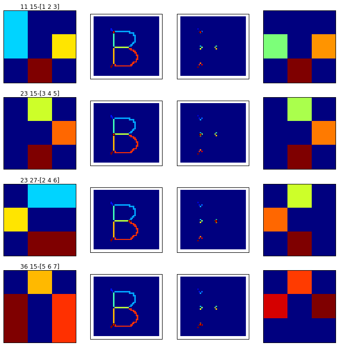
endpoints (blue), branched points (green)

Endpoints Spectrum :

The skeleton of the hand has two endpoints close to top of each fingers, as it would be fine to have one endpoint per finger, let's prune the skeleton to meet this condition. This can be achieved after some trial, however if robust features could be found from the skeleton a systematic method is needed. So, let's prune the skeleton until it has no endpoint and count the number of pruning step necessary:
From the curve, the hand skeleton has 13 endpoints before any pruning, after 40 pruning steps, it has 6 endpoints. Around 90 pruning steps are necessary to remove all endpoints. By only looking at their curve, the hand shaped silhouette and the fish shaped silhouette are different.

Endpoints spectrum resists to scale variation after normalization:

As scale invariance is a nice feature, let's see what is happening when the scale of the shape is successively reduced by a factor of 0.9², 0.7², 0.5², 0.3²:
From the images above, it is clear that  the skeleton resists to scale variations but as the skeleton becomes smaller  less pruning steps are necessary to "burn" it to the last pruned pixels set. So let's norme the pruning steps by the initial skeleton size such for 0 pruning step, the normed pruning step is 100. As the size of the hand shaped silhouette decreases (from 81%, 49%, 25%, 9% of the original size), the endpoints spectrums  remain comparable:

Endpoints spectrum of similar shapes are similar:

How does the curve behave with similar shapes? Let's compare the endpoints spectrum of the serie of six hands:

The spectrums seem to resist to shape rotation (hand, hand-10°, hand90°) and to moderate shape deformation (hand-bent1,2). The sketch-hand silhouette is a right hand and its spectrum is comparable to the other spectrums which corresponds to left hands, so the endpoints spectrum is symetry invariant too.

Deriving a features vector from endpoints spectrum:

If shapes should be classified according to their topology, the whole endpoints spectrum is not necessary and only the transitions may be retained. Taking a  hypothetical skeleton whose endpoints spectrum before normalization is:
  • For 7 prunings the skeleton has 0 endpoints
  •       6                                        1
  •       2                                        3
  •       0                                        4
So a possible features vector would be:
(7,6,-1,2,0)
The value -1 indicates that the value 2 endpoints is missing. In the python script, the endpoints spectrum is coded as two lists:
             end_points_test   = [4,3,3,1,1,1,1,0]
             pruning_steps_test = [0,1,2,3,4,5,6,7]

A python function taking the steps list and the endpoints (spectrum) list yields a features vector :
def EPSpectrumToFeatures(steps, spectrum):
    '''
          eptest   = [4,3,3,1,1,1,1,0]
          pruntest = [0,1,2,3,4,5,6,7]
the returned vec:[7,6,-1,2,0] which means:
    0 enpoints -> 7 prunings necessary
    1 endpoint -> 6 prunings
    4 endpoints-> 0 pruning (initial skeleton size)
'''
     values = set(spectrum)
    feat_vect = [-1]*(len(values)+1)
    spec = np.asarray(spectrum)
    for epn in values:
        indexmin = np.where(spec == epn)[0][-1]
        feat_vect[epn] = steps[indexmin]
    return feat_vect
Supposing now the the skeleton size is 25, let's normalise the pruning steps as follow: 
  
 normed_pruning_steps_test = [100*(1-i/25.0) for i in pruntest] 

The endpoints spectrum is:

Let's take a normalised endpoints spectrum:
  • normedsteps = [100.0, 96.0, 92.0, 88.0, 84.0, 80.0, 76.0, 72.0]
  • endpoints = [4, 3, 3, 1, 1, 1, 1, 0] 
 
And let's submit it the previous function :

EPSpectrumToFeatures(normedsteps, endpoints)

 The function yields the vector:
[72.0, 76.0, -1, 92.0, 100.0]
which means that the skeleton has:
  • 0 endpoint for a normed number of  prunings of 72%
  • 1  ---------------------------------------------------------------------------76%
  • no 2 endpoints, set normed number of  prunings to -1
  • 3 -------------------------------------------------------------------- 92%
  • 4 ------------------------------------------------------------------ 100%
The different endpoints spectrum curves suggest that the vector could used for classifying 2D binary shapes.

A feature vector from a real shape:

Let's consider the shape of a hand:
Its endpoints spectrum (normalised by skeleton size or not) was calculated and a feature vector was derived and displayed (red) with the spectrum:
Left: raw endpoints spectrum (blue) and its feature vector (red). Right: Normed endpoints spectrum and its feature vector, for 100% of the skeleton size, the skeleton has 14 endpoints, for ~94% the skeleton has 7 endpoints and for 83% of the skeleton size the skeleton has no endpoint.
For a larger number of image a python class, called Shape was written. It is instantiated as follow: 
shape= Shape(image)

The feature vector can be computed by:

vector = shape.End_Points_Features(normed = True)
or by:
vector = shape.End_Points_Features(normed = False)

Feature vectors from 216 images :

216 images of small 2D binary images (silhouettes) [Sharvit et al.] were used to derive feature vectors. This set of images consists in 18 type of silhouettes with 12 instance of each. For example, there are 12 birds silhouettes:
Prior any kind of classification the 216 normed feature vectors were aligned for visual inspection:
Some silhouettes, as the Bone silhouettes seems to show some intra-class structure, while Brick and Camel silhouettes seems different.

ipython notebook (updated 24/05/2013):

All the  tasks were performed in a ipython notebook available here.


Tuesday, April 9, 2013

Detecting end points or branched points from the skeleton of a single chromosome

The end-points or the branched-points from the skeleton of a single chromosome can be extracted using mathematical morphology operators implemented in mahotas.
Two images of metaphasic human chromosomes hybridized with a Cy3-telomeric PNA probe and  counterstained with DAPI, were used.
 
False color DAPI image
False color telomeres image
The location of a chromosome was identified, some preprocessing step were performed to segment the chromosome (hi-pass filtering followed by a simple thresholding).
The end-points, the branching points are extracted from the skeleton with a hit-or-miss operator implemented in mahotas, then overlayed on the original chromosome image.
The contour of the segmented telomeres are also overlayed:
Depending on the amount of high-pass filtering the chromosome skeleton fit the chromosome axis or the chromatids:
Skeletonization after "low" high-pass filtering
Skeletonization after a stronger high-pass filtering
In both cases, the skeleton is displayed in red, the branched-points in green, the end-points in blue, the chromosome contour in magenta, and finally the telomeres in yellow.
To run the code (python 2.7), the path to the images must be modified and mahotas and pymorph must be installed.
Download code

Friday, February 15, 2013

Chromosomal shapes classification by Linear Discriminant Analysis with R

Features were tested to distinguish overlapping chromosomes from single chromosomes and from nuclei or from image segmentation artefacts:
Two overlapping chromosomes
Those features are:
  • The chromosomes size (normalized by the image size).
  • The ratio of chromosome area by the convexhull area

convex hull of overlapping chromosomes


  • The non chromosomal domains area in a convex hull. The four largest (normalized by the convex hull area) non chromosomal domains  were kept:
Areas of size h1, h2, h3, h4
Chromosomes from twelve metaphases were classified with minikar. In a previous post, an isolated result indicated that these six features doesn't seem to distinguish the different particles.
Each observation falls in one of the four categories (single, cluster, nuclei, dust). 451 observations were used  to build a trained set by linear discriminant analysis (lda) according to this example.

Prior  lda, a pairs plot can be done where each color corresponds to one category (single chromosome, touching chromosomes, nuclei, dusts):
Pairs plot between the six variables: var1 (area), var2 (area/convexhull), var3,4,5,6 (area of h1,h2,h3, 4)
The observations seem more or less clustered according to the pair of variables considered. The first plot (ratio ~ area) was previously done showing an overlay between the single and cluster categories. LDA was used here as a black box, with the aim to know if a good classification can be achieved and how good are the features.

Pratically the work was done with R within rstudio. Data were downloaded from github, assembled into a data frame and analysed. LDA performed here data reduction from six variables to three (LD1, LD2, LD3) and when the variable LD1 is plot against LD2, it yields:
Clearly showing separated clusters. The most populated (blue), corresponds to the single chromosomes, pink dots are the touching chromosomes, the green dots and the red dots are probably the nuclei and the dusts repectively (I have to check how to put a legend in that plot).
However, the classification is still imperfect:

 28/80 touching chromosomes and 6/30 nuclei  were classified as single chromosomes. No single chromosomes were misclassified.

# Download features and label file from github
require(RCurl)
library(RCurl)
feat_prefix <-'jp-Jpp48-'
sufix <- '-DAPI.csv'
lab_prefix <- 'shapeCateg-jp-Jpp48-'
webpath <- 'https://raw.github.com/jeanpat/pyFISH/master/GUI/karyotyper/example%20classification/source%20data/'
files <- list(1, 2, 3, 5, 6, 7, 8, 9, 10, 11, 14, 15)
data <- data.frame()
for (file in  files){
  featname <- paste(webpath,'features/',sep='')
  featname <- paste(featname,feat_prefix,as.character(file),sufix,sep='')
  labname <- paste(webpath,'labels/',sep='')
  labname <- paste(labname, lab_prefix, as.character(file),sufix,sep='') 
  print (featname)
  print (labname)
  features <- getURL(featname)
  labels <- getURL(labname)
  features <- read.table(text = features, sep = ';')
  labels <- read.table(text = labels, sep = ';')
  #print (str(features))
  # add metaphase number ()
  features$metaphase <- file
  #merge features and labels
  features <- cbind(features,labels)
  data <- rbind(data, features)
  }
#print (head(data))
#remove duplicate column
data[,9] <- NULL
#rename columns
colnames(data)[1]<-'particle'
colnames(data)[2]<-'area'
colnames(data)[3]<-'ratio'
colnames(data)[4]<-'h1'
colnames(data)[5]<-'h2'
colnames(data)[6]<-'h3'
colnames(data)[7]<-'h4'
colnames(data)[8]<-'meta'
colnames(data)[9]<-'type'
print (str(data))
pairs(cbind(data$area,data$ratio,data$h1,data$h2,data$h3,data$h4),col=c("red","blue","green","orange")[data$type],upper.panel=NULL,)
#
# Linear discriminant analysis was performed as explained:
#
# http://www.youtube.com/watch?v=bOSVge_PQF4
#
library(lattice)
library(MASS)
chr.lda <- lda(type~area+ratio+h1+h2+h3+h4,data=data)
summary(chr.lda)
chr.pred <- predict(chr.lda)
ErrorTable<-table(data$type,chr.pred$class)
print (ErrorTable)
lda.tmp <- data.frame(chr.pred$x,class=chr.pred$class)
xyplot(LD1~LD2,data=lda.tmp, group=class)
Created by Pretty R at inside-R.org