Wednesday, April 20, 2011

Hit or miss: skeleton and convex hull with Python

The following script is used to detect both branching points (green) and endpoints (blue)in skeletons (red) of touching and overlapping chromosomes, before and after high pass filtering of the image of the chromosomes.

Hit and miss morphological operator is also used to compute the convex hull of a particle. I try to implement the algorithm without success, the convex hull calculated (red) is not different from the initial binary particle (white):
Upper and middle image: Skeleton analysis. Lower image: fail to produce a convex hull (red)
 The set of structuring elements used in the convex hull function, corresponds to all the possible corners in 3x3 pixel array.


Convex hull algorithm (II) :
The first trial was not successful due to a boolean type issue. I tried to implement the algorithm again according to the definition found in Gonzalez & Woods, "Digital Image Processing", using the hit or miss operator provided by the mahotas library.
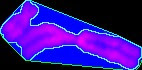
Lower image:result in red of the convex hull found
Clearly the function ConvexHull_2, I implemented, gives a wrong result. 
For comparison, the convex hull obtained with ImageJ is:
Convex hull (blue)
De DIP4FISH
However, the result seems to be correct on the "west" side or on the "east" side of the image whereas "North" and "South" are wrong. The structuring elements may be implicated, or not .... (to be continued).

def ConvexHull_2(bim):
    ''' 
    From Gonzalez & Woods p545 (Addison Wesley 1992), the algorithm is:
        X(i,0)=A        
        X(i,k)=[X(i,k-1)*B(i)] u A
        D(i)=X(i,conv) conv such X(i,k)=X(i,k-1)
        k=1,2,3,....
        i=1,2,3,4 :one of the four structuring element B of type III
        convexhull of A: C(A)=u(from i=1 to 4) D(i)
        *: hit or miss operator
        u:union
    '''
    #
    #           3x3 structuring elements: 
    #   0:no pixels; 1: one pixel; 2:don't care
    #
    cornerS=np.array([[2,2,2],
                      [2,0,2],
                      [1,1,1]])
    
    cornerE=np.array([[2,2,1],
                      [2,0,1],
                      [2,2,1]])
    
    cornerN=np.array([[1,1,1],
                      [2,0,2],
                      [2,2,2]])
    
    cornerW=np.array([[1,2,2],
                      [1,0,2],
                      [1,2,2]])
    def countTruePix(bim):
        '''bim must be a binary array 
      Counts the occurence of True (pixel)'''
        return np.sum(bim[:,:]==True)
    
    def HitMissConfigUpToConv(bim,config):
        '''
        config is the "i" of the algo
        '''
        if config=="N":B=cornerN
        if config=="W":B=cornerW
        if config=="S":B=cornerS
        if config=="E":B=cornerE
        X=bim
        idempotence=False
        k=1
        while not(idempotence):
            size=countTruePix(X)
            hitpoints=mah.morph.hitmiss(X.astype(bool),B)
            X=X+hitpoints
            newsize=countTruePix(X)
            #size==newsize supposes that idempotence (convergence) is reached
            #this may not be true:same size but different shape
            idempotence=(newsize-size==0)
            k=k+1
        return X
    #starts here
    A=bim
    D1=HitMissConfigUpToConv(A,"N")
    D2=HitMissConfigUpToConv(A,"W")
    D3=HitMissConfigUpToConv(A,"S")
    D4=HitMissConfigUpToConv(A,"S")
    return D1+D2+D3+D4

Sunday, April 17, 2011

Analysis of the orientation of a particle by erosion

A metaphase image contains randomly oriented chromosomes, possibly overlapping and sometime nuclei. An automatic cytogenetic application should be able to detect and resolve overlapping chromosomes, to display chromosomes vertically for further karyotyping.

A step in the chromosome shape analysis, is to detect the chromosome orientation. The following script takes an isolated chromosome image, thresholds it, counts how many vertical erosions are necessary to erase the particle, rotates the image and do it again for all the rotation angle from 0° to 180°.
Result:
 Several kind of particles were tested: a small chromosome, a metacentric one, two overlapping chromosomes and a nuclei. A peak in the curve corresponds to the main particle orientation in the image. Overlapping chromosomes may yield a two peaks curve.

One peak curve for the above chromosome.A rotation of 50°, yields the highest resistance to erosion.
A small chromosome
.
Signature of a small chromosome

Signature of overlapping chromosomes
Nuclei
Signature of a nuclei. 130 iterations are necessary to erase the particle, compared to 22 for the small chromosome.

Wednesday, April 13, 2011

Detecting end points in a skeleton

In order to detect overlapping chromosomes, or to analyse the shape of a chromosome it could be useful to analyse the shape of the particle skeleton.
In the previous post hit-or-miss morphological operator, with the proper structuring element, detects branched points of a skeleton. Those points are indicated to classify overlapping chromosomes, even if pruning the skeleton might be necessary.
Here, with other structuring elements, hit-or-miss operator detects the end points of particle constituted of overlapping and touching chromosomes.

Download python code
 Lower image: green points (branched points of the skeleton), blue points (end points of the skeleton)

Tuesday, April 12, 2011

Detecting branched points in a skeleton

 
The image of a segmented chromosome (top left) is thresholded (top right) then used to calculate a skeleton with mahotas.thin() (lower left). The skeleton branched points  are detected by a hit-or-miss operator (lower right).
The python script depends on mahotas, pymorph, scipy.

Thursday, April 7, 2011

Testing hit or miss with mahotas 0.6.4

Mahotas 0.6.4 is out. I upgrade my distribution with:
sudo easy_install --upgrade mahotas

Let's try to analyse a chromosome skeleton by hit and miss to detect end-points :
Top left:original image. Top right:thresholded image.Bottom left:skeleton. Bottom right:end-points
The skeleton of the binary image is build with pymorph.skelm(), then submitted to hit or miss transformation.
Strangely the skeleton is not a one connected component particle as it was the case here.
The python script is:
# -*- coding: utf-8 -*-
"""
Created on Thu Apr  7 10:08:16 2011

@author: Jean-Patrick Pommier
"""
import mahotas as mah
import pymorph as pm
import numpy as np
import pylab as plb
import os

user=os.path.expanduser("~")
workdir=os.path.join(user,"Applications","ImagesTest","jp","Jpp48","13","DAPI","particules")
file="part14.png"
#structuring elements
N=np.array([[0, 0, 0], [0, 1, 0], [0, 1, 0]])
NW=np.array([[0, 0, 0], [0, 1, 0], [1, 0, 0]])
W=np.array([[0, 0, 0], [1, 1, 0], [0, 0, 0]])
SW=np.array([[1, 0, 0], [0, 1, 0], [0, 0, 0]])
S=np.array([[0, 1, 0], [0, 1, 0], [0, 0, 0]])
SE=np.array([[0, 0, 1], [0, 1, 0], [0, 0, 0]])
E=np.array([[0, 0, 0], [0, 1, 1], [0, 0, 0]])
NE=np.array([[0, 1, 0], [0, 1, 0], [0, 0, 1]])
square=pm.asbinary(np.array([[1, 1, 1], [1, 1, 1], [1, 1, 1]]))
if __name__ == "__main__":
    complete_path=os.path.join(workdir,file)
    i1=mah.imread(complete_path)
    bi1=(i1>0)
    sk=pm.skelm(bi1)
    p0=mah.morph.hitmiss(sk,N)
    p1=mah.morph.hitmiss(sk,NW)
    p2=mah.morph.hitmiss(sk,W)
    p3=mah.morph.hitmiss(sk,SW)
    p4=mah.morph.hitmiss(sk,S)
    p5=mah.morph.hitmiss(sk,SE)
    p6=mah.morph.hitmiss(sk,E)
    p7=mah.morph.hitmiss(sk,NE)
    endpoints=p0+p1+p2+p3+p4+p5+p6+p7
    plb.gray()
    plb.subplot(2,2,1)
    plb.imshow(i1,interpolation=None)
    plb.subplot(2,2,2)
    plb.imshow(bi1,interpolation=None)
    plb.subplot(2,2,3)
    plb.imshow(sk,interpolation=None)
    plb.subplot(2,2,4)
    plb.imshow(endpoints,interpolation=None)
    plb.show()

Second trial: let's label the skeleton:
In the second trial, I only try to label the skeleton.


# -*- coding: utf-8 -*-
"""
Created on Thu Apr  7 10:08:16 2011

@author: Jean-Patrick Pommier
"""
from scipy import ndimage as nd
import mahotas as mah
import pymorph as pm
import numpy as np
import pylab as plb
import os

user=os.path.expanduser("~")
workdir=os.path.join(user,"Applications","ImagesTest","jp","Jpp48","13","DAPI","particules")
file="part14.png"
#structuring elements
N=np.array([[0, 0, 0], [0, 1, 0], [0, 1, 0]])
NW=np.array([[0, 0, 0], [0, 1, 0], [1, 0, 0]])
W=np.array([[0, 0, 0], [1, 1, 0], [0, 0, 0]])
SW=np.array([[1, 0, 0], [0, 1, 0], [0, 0, 0]])
S=np.array([[0, 1, 0], [0, 1, 0], [0, 0, 0]])
SE=np.array([[0, 0, 1], [0, 1, 0], [0, 0, 0]])
E=np.array([[0, 0, 0], [0, 1, 1], [0, 0, 0]])
NE=np.array([[0, 1, 0], [0, 1, 0], [0, 0, 1]])
square=pm.asbinary(np.array([[1, 1, 1], [1, 1, 1], [1, 1, 1]]))
if __name__ == "__main__":
    complete_path=os.path.join(workdir,file)
    i1=mah.imread(complete_path)
    bi1=(i1>0)
    sk=pm.skelm(bi1)
    sklabel,npart=nd.label(sk)
    print npart
    p0=mah.morph.hitmiss(sk,N)
    p1=mah.morph.hitmiss(sk,NW)
    p2=mah.morph.hitmiss(sk,W)
    p3=mah.morph.hitmiss(sk,SW)
    p4=mah.morph.hitmiss(sk,S)
    p5=mah.morph.hitmiss(sk,SE)
    p6=mah.morph.hitmiss(sk,E)
    p7=mah.morph.hitmiss(sk,NE)
    endpoints=p0+p1+p2+p3+p4+p5+p6+p7
    plb.gray()
    plb.subplot(2,2,1)
    plb.imshow(i1,interpolation=None)
    plb.subplot(2,2,2)
    plb.imshow(bi1,interpolation=None)
    plb.subplot(2,2,3)
    plb.imshow(sk,interpolation=None)
    plb.subplot(2,2,4)
    plb.jet()
    plb.imshow(sklabel,interpolation=None)
    plb.show()